Shapelez 28 мая 2021 в 17:52

Overview of Morris's counters

7 мин

1.3K

Блог компании Qrator LabsВысокая производительность*Алгоритмы*Математика*

An artist's concept showing counting of elements in a stream with limited resources

_{We are glad to present you an article written by Qrator Labs' engineer Dmitry Kamaldinov. If you want to be a part of our Core team, write us at}_{hr@qrator.net}_.

1 Introduction

On implementing streaming algorithms, counting of events often occurs, where an event means something like a packet arrival or a connection establishment. Since the number of events is large, the available memory can become a bottleneck: an ordinary -bit counter allows to take into account no more than 2^n - 1 events.
One way to handle a larger range of values using the same amount of memory would be approximate counting. This article provides an overview of the well-known Morris algorithm and some generalizations of it.

Another way to reduce the number of bits required for counting mass events is to use decay. We discuss such an approach here [3], and we are going to publish another blog post on this particular topic shortly.

In the beginning of this article, we analyse one straightforward probabilistic calculation algorithm and highlight its shortcomings (Section 2). Then (Section 3), we describe the algorithm proposed by Robert Morris in 1978 and indicate its most essential properties and advantages. For most non-trivial formulas and statements, the text contains our proofs, the demanding reader can find them in the inserts. In the following three sections, we outline valuable extensions of the classic algorithm: you can learn what Morris's counters and exponential decay have in common, how to improve the accuracy by sacrificing the maximum value, and how to handle weighted events efficiently.

2 Probabilistic Counting, problems of the trivial approach

The main idea of probabilistic counting is taking into account the next event with a certain probability. Let us first consider an example with a constant update rate:

$\begin{equation*} C_{n+1} = \left\{\begin{array}{ll} C_n + 1 & \textit{with probability $p = const$} \\ C_n & \textit{with probability $1-p$.} \end{array}\right. \end{equation*}$

Where C_n denotes the counter value after the th update attempt. It is easy to see that C_n gives the number of successes among nn independent Bernoulli trials. In other words, C_n has a binomial distribution:

$\begin{align*} C_n \sim Bin(&n, p) \\ {\sf E} C_n = &np \\ {\sf D} C_n = &np(1-p). \end{align*}$

The problem we are to solve is to estimate the actual number of events given only the random value C_n obtained accordingly to the described update rule. It is natural to use $\widehat{n}(C) := C/p$ as an estimator, since we know C_n = np on average.

The described approach has several drawbacks: first, it allows to count up to 1/p = const times larger numbers comparing to the ordinary incremental counter, which is still noticeably less than, as we will see below, we get with Morris's counters. Second, the relative error is high for small . For example, if n = 1 it is up to 100%. The coefficient of variation can estimate the relative error:

$\begin{align*} {\sf CV}\widehat{n}(C_n) = \frac{\sqrt{{\sf D}\widehat{n}(C_n)}}{{\sf E} \widehat{n}(C_n)} = \sqrt{\frac{1-p}{pn}}. \end{align*}$

3 Morris's counters

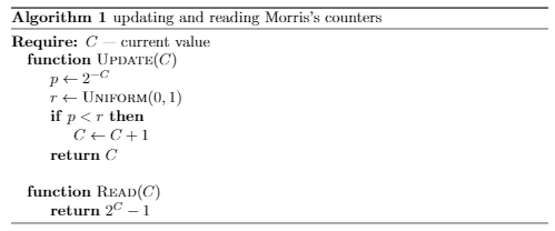
The Morris's counter updates with a probability dependent on the current value: the first update occurs with a probability of 1, the next with 1/2, then 1/4, etc.:

$\begin{equation*} C_{n+1} = \left\{\begin{array}{ll} C_n + 1 & \textit{with probability $2^{-C_n}$} \\ C_n & \textit{with probability $1 - 2^{-C_n}$.} \end{array}\right. \end{equation*}$

How to estimate the number of events by the current counter value? Updating the counter from to x + 1 occurs on average after 2^x iterations, hence a reasonable estimator would be

$\widehat{n}(C) := \sum_{i=0}^{C-1} 2^i = 2^C - 1$

The most important properties of this estimator are the following:

it is unbiased, that is, the estimate after nn updates is on average ,

Proof

$\begin{align*} {\sf E}\left(2^{C_n} | C_{n-1} = y\right) =& \underbrace{2^{y + 1} 2^{-y}}_{\textit{increment happened}} + \underbrace{2^y (1 - 2^{-y})}_{\textit{no change}} = 2^y + 1 \implies \\ {\sf E}(2^{C_n}|C_{n-1}) =& 2^{C_{n-1}} + 1 \implies {\sf E}2^{C_n} = {\sf E}2^{C_{n-1}} + 1 = {\sf E}2^{C_{n-2}} + 2 = \dots \end{align*}$

At the very beginning, the counter value is 0: C_0 = 0 then ${\sf E}2^{C_0} = 2^{0} = 1$ , so ${\sf E} 2^{C_n} = \dots = n + 1$ . Finally, ${\sf E}\widehat{n}(C_n) = {\sf E}2^{C_n} - 1 = n$ .

and its relative error is independent of .

Proof

First, let's calculate the variance of $\widehat{n}(C_n)$ . According to the well-known formula, ${\sf D}\widehat{n} = {\sf E}\widehat{n}^2 - ({\sf E}\widehat{n})^2$ . We already know ${\sf E}\widehat{n}(C_n) = n$ . It remains to get ${\sf E}\widehat{n}(C_n)^2$ . Notice, that

$\begin{align*} {\sf E}\left(2^{C_n} - 1\right)^2 = {\sf E}2^{2C_n} - 2(n+1) + 1 = {\sf E}2^{2C_n} - 2n - 1. \end{align*}$

So, we are only to find ${\sf E}2^{2C_n}$ .

$\begin{align*} {\sf E}\left(2^{2C_n} | C_{n-1} = y\right) &= \underbrace{2^{2(y + 1)} 2^{-y}}_{\textit{increment happened}} + \underbrace{2^{2y}(1 - 2^{-y})}_{\textit{no change}} = \\ = 3 \cdot 2^y +2^{2y} &\implies {\sf E}\left(2^{2C_n} | C_{n-1}\right) = 3 \cdot 2^{C_{n-1}} + 2^{2C_{n-1}} \implies \\ {\sf E} 2^{2C_n} = 3n &+ {\sf E}2^{2C_{n-1}} = 3n + 3(n-1) + {\sf E}2^{2C_{n-2}} = \dots = \sum_{i=1}^n 3i \end{align*}$

Finally,

$\begin{equation*} {\sf D}\widehat{n}(C_n) = \frac{3n(n+1)}{2} - 2n - 1 - n^2 = \frac{n^2 - n - 2}{2} \end{equation*}$ $\begin{equation*} {\sf CV}\widehat{n}(C_n) = \frac{\sqrt{{\sf D}\widehat{n}(C_n)}}{{\sf E}\widehat{n}(C_n)} = \sqrt{\frac{n^2-n-2}{2n^2}} \sim \frac{1}{\sqrt{2}}. \end{equation*}$

And also, we can bound tail probabilities by Chebyshev's inequality:

$\begin{align*} {\sf P}(|\widehat{n}(C_n) - n| \ge \varepsilon n) \le \frac{{\sf D}\widehat{n}(C_n)}{\varepsilon^2n^2} \sim \frac{1}{2\varepsilon^2}. \end{align*}$

Thus, the relative error of the number of events estimate is bounded, approximately constant and almost independent of .

If we are restricted with ${\bf X}$ bits of memory, the event number range we can cover is ${\bf N}_{max} = 2^{2^{\bf X}} - 1$ . In other words, $\mathcal{O}(\log \log n)$ bits are sufficient to account up to events!

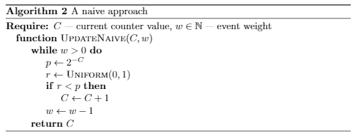
Figure 1: relative error of the event number estimate while using binomial counters and Morris's counters (the plot was obtained by sample_size=100 times simulating the evolution process of the counter and mapping each point n onto the average relative error of estimate at this point)

4 Weighted updates

Morris's counters can be used to count weighted events: for example, to sum up the sizes of incoming packets. The simplest way — updating the counter <event weight> times — leads the update complexity to be linear in weight.

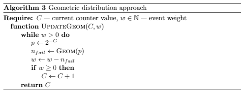
Note that at each moment, we know how the number of update failures before the subsequent success is distributed; this is the geometric distribution:

$\begin{align*} {\sf P}(n_{fail} = k) = (1 - 2^{-C})^k 2^{-C} \implies n_{fail} \sim Geom(2^{-C}). \end{align*}$

Given this fact, we can speed up the algorithm by immediately skipping all consecutive unsuccessful update attempts:

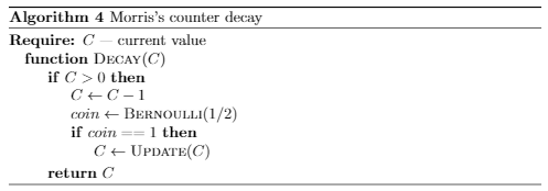
5 Decay

There is often a need to take into account the most recent events with a higher priority. For instance, when looking for intensive keys in a stream, we might be more interested in detecting keys intense right now, rather than ones having a high average intensity due to the events in the past. In the article [3], we discussed the decay counters explicitly designed for this purpose. Another prerequisite for some form of decay is that despite the super-economical use of memory, even Morris's counters once may overflow. Fortunately, it turns out Morris's counters can also decay, moreover, it is very similar to EMA but much more efficient.

The basic idea is quite simple: we periodically subtract from the counter. Recall the counter value of estimates the number of events as $\sum_{i = 0}^{C-1} 2^i = 2^C - 1 =: n_0$ .

Accordingly, after subtracting the estimate becomes $2^{C-1} - 1 = \frac{1}{2} n_0 - \frac{1}{2}$ .

In other words, subtracting decreases the estimate by a factor of $\sim 2$ ! We can achieve exactly times decrease by updating the counter with probability $\frac{1}{2}$ immediately after subtracting :

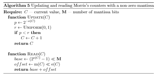
6 Mantissa and exponent

Consider the following generalization of Morris's counters: the probability of an update is halved not on every successful update, but on every ${\bf X}$ updates. One possible implementation of this approach would be splitting the counter bits into two parts: exponential, responsible for the probability, and significand, counting the number of successful updates within the current probability (the notions are taken from floating point arithmetic).

Figure 2: splitting counter bits into E=3 exponential and M=5 significand

Let us introduce the notation for the exponential and significand parts:

$\begin{align*} {\rm e}(C) &= C \gg {\bf M} \\ {\rm m}(C) &= C \& (2^{\bf M} - 1). \end{align*}$

Now the update rule and the estimator of the number of events are written as follows:

$\begin{align*} C_{n+1} &= \left\{\begin{array}{ll} C_n + 1, & \textit{with probability $2^{-{\rm e}(C)}$} \\ C_n, & \textit{with probability $1 - 2^{-{\rm e}(C)}$} \end{array}\right. \\ \widehat{n}(C) &= (2^{{\rm e}(C)} - 1)2^{\bf M} + 2^{{\rm e}(C)}{\rm m}(C). \end{align*}$

For example, on figure 2 counter value is C = 89 , the mantissa and exponent are equal to ${\rm m} = 25$ and ${\rm e} = 2$ correspondingly. So the event number estimate is $\widehat{n} = (2^2 - 1) \times 2^5 + 2^2 \times 25 = 196$ .

With such a partition, the bits of the exponent are responsible for the covered range of the number of events, and the bits of the mantissa determine the accuracy of the estimate (these claims are described in detail below). The best partition of the counter bits depends on the application; we suggest giving as many bits to the mantissa as possible, but with enough exponential bits to cover the target value range.

The described variant of Morris's counters has the following properties:

the covered range of values is

$\begin{align*} {\bf N}_{max} = 2^{2^{\bf E} + {\bf M}} - \left(2^{2^{\bf E} - 1} + 2^{\bf M}\right); \end{align*}$

Proof

The covered range is easy to get by substituting the maximum possible values ${\rm m} = 2^{\bf M} - 1$ and ${\rm e} = 2^{\bf E} - 1$ into the estimator $\widehat{n}$ :

$\begin{align*} {\bf N}_{max} = \left(2^{2^{\bf E} - 1} - 1\right)2^{\bf M} + 2^{2^{\bf E} - 1}\left(2^{\bf M} - 1\right) = 2^{2^{\bf E} + {\bf M}} - \left(2^{2^{\bf E} - 1} + 2^{\bf M}\right) \end{align*}$

a new estimator $\widehat{n}$ is also unbiased: ${\sf E}\widehat{n}(C_n) = n$ ;

Proof

Similarly to the proof of the statement for the ordinary Morris's counters, we calculate the conditional expectation ${\sf E}(C_n | C_{n - 1} = y)$ . And we will do it separately for $y \equiv -1 \pmod{2^{\bf M}}$ (the probability of the update changes on success) and $y \not\equiv -1 \pmod{2^{\bf M}}$ .

$\begin{align*} y \not\equiv -1 \pmod{2^{\bf M}} &\implies {\rm e}(y + 1) = {\rm e}(y), \quad {\rm m}(y + 1) = {\rm m}(y) + 1 \\ &\implies \widehat{n}(y + 1) = \widehat{n}(y) + 2^{{\rm e}(y)} \\ y \equiv -1 \pmod{2^{\bf M}} & \implies {\rm e}(y + 1) = {\rm e}(y) + 1,\\ &\phantom{\implies} \phantom{Z} {\rm m}(y) = 2^{\bf M} - 1, \quad {\rm m}(y + 1) = 0 \implies \\ \widehat{n}(y + 1) = \widehat{n}(y) &- 2^{{\rm e}(y)}\left(2^{\bf M} - 1\right) + 2^{{\rm e}(y) + {\bf M}} = \widehat{n}(y) + 2^{{\rm e}(y)} \end{align*}$

In both cases

$\begin{align*} {\sf E}\left(2^{C_n} | C_{n-1} = y\right) &= \widehat{n}(y)\left(1 - 2^{-{\rm e}(y)}\right) + \left(\widehat{n}(y) + 2^{{\rm e}(y)}\right)2^{-{\rm e}(y)} = \widehat{n}(y) + 1. \end{align*}$

the coefficient of variation (and the relative error) gets even smaller! We do not know its exact value, but there is a bound:

$\begin{align*} {\sf CV}\widehat{n}(C_n) \le 2^{-\frac{{\bf M} + 1}{2}}. \end{align*}$

(recall the analogous value for classic Morris's counter is $2^{-1/2}$ )

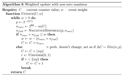
Weighted update and decay algorithms will also change slightly.

Similarly to the approach described in Section 4, to perform a weighted update efficiently, we are to figure out how many update attempts are needed to change the probability. Formerly, without the mantissa, the probability changes on each successful update, but now it changes after every $2^{\bf M}$ updates. So we need the distribution of the number of Bernoulli trials (the required number of events), among which there are precisely $2^{\bf M}$ successful ones. This distribution is called negative binomial.

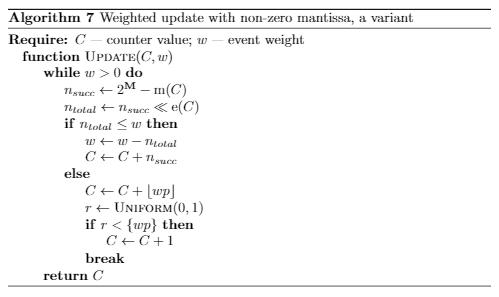
_Remark._{Actually, there are several definitions of the negative binomial distribution. We will use the one that claims it as a distribution of the number of failures with a given number of successes. Then, to get the number of events, we need to add the number of successes to the random value:}

$\begin{align*} n \sim \underbrace{NegativeBinomial\left(2^{-{\rm e}(C)}, 2^{\bf M} - {\rm m}(C)\right)}_{\textit{failures}} + \underbrace{\left(2^{\bf M} - {\rm m}(C)\right)}_{\textit{successes}}. \end{align*}$

In order to avoid generating the negative binomial distribution, one can simplify the algorithm by just using the mean of this distribution:

To perform the decay, we subtract from the exponential part (in other words, $2^{\bf M}$ from the counter value). Then

$\begin{align*} \widehat{n}\left(C - 2^{\bf M}\right) = (2^{{\rm e}(C) - 1} - 1)2^{\bf M} + 2^{{\rm e}(C) - 1}{\rm m}(C) = 1/2\widehat{n}(C) - 2^{{\bf M}-1}. \end{align*}$

Note that for ${\bf M}>0$ (namely, this case is studied in this section) $2^{{\bf M}-1} \in \mathbb{N}$ . Therefore, the estimate can be corrected by updating by $2^{{\bf M}-1}$ :

7 Conclusion

Morris's counters are awesome! Use them!

The last section does not contain practical results, but ...

8 Generalized Probabilistic Counters

In general, the rule for updating the counter is determined by the probability function $F : C \mapsto [0, 1]$ :

$\begin{equation*} C_{n+1} = \left\{\begin{array}{ll} C_n + 1 & \textit{with probability $F(C_n)$} \\ C_n & \textit{with probability $1 - F(C_n)$.} \end{array}\right. \end{equation*}$

In the case of Morris's counters $F(C_n) = 2^{-C_n}$ . When studying probabilistic counters, we tried to take a linear probability function: $F(C_n) = 1 - \frac{C_n}{C_{max}}$ ( $C_{max}$ — some constant, the upper bound of the counter).

This had led to some interesting results, which are summarized in this section.

Before presenting these results, let us recall two mathematical entities. A complete symmetric homogeneous polynomial of degree in variables $x_1, \dots, x_m$ is the sum of all possible monomials of degree in these variables with coefficients :

$\begin{align*} \mathcal{H}_n(x_1, \dots x_m) = \sum_{\begin{array}{cc} & 0 \le i_j \le n \\ & i_1 + \dots + i_m = n \end{array}} x_1^{i_1} \cdots x_m^{i_m}. \end{align*}$

Another construction that we need is the Stirling number of the second kind. One of the ways to define this number is combinatorial: the Stirling number of the second kind $\genfrac\{\}{0pt}{}{n}{m}$ is the number of partitions of the nn-element set into mm non-empty subsets. Stirling numbers are associated with complete symmetric homogeneous polynomials:

$\begin{align*} \genfrac\{\}{0pt}{}{n+m}{m} = \mathcal{H}_m(1, 2, \dots, m). \end{align*}$

With the help of $\mathcal{H}$ , we can write in general form the probability of counter value after updates being equal to

$\begin{align*} {\sf P}(C_n = m) = \left[\prod_{k=0}^{m-1} F(k) \right] \mathcal{H}_{n-m}(1-F(1), \dots 1-F(m)). \end{align*}$

This formula is easy to prove by induction. However, it can also be deduced from simple combinatorial reasoning: in fact, it says that in order to get the value of , successful updates are needed: from to , from to , and etc., — the factor $\prod_{k=0}^{m-1} F(k)$ stands for this;

and n-m unsuccessful, which can be logically divided into groups: i_1 failed updates from to , i_2 from to , and so on, which is expressed as $\mathcal{H}_{n-m}$ .

Finally, when using the linear probability function $F(C) = 1 - \frac{C}{C_{max}}$ , the probability takes the form

$\begin{equation*} {\sf P}(C_n = m) = \genfrac\{\}{0pt}{}{n}{m} \frac{C_{max}!}{(C_{max} - m)!C_{max}^n}. \end{equation*}$

That is the exciting result announced above. We noticed the Stirling number in the probability value quite accidentally and still do not know whether it is possible to justify its presence by combinatorial reasoning (relying on its combinatorial definition). One another question is whether there is also a nice formula for ${\sf P}(C_n = m)$ in the case of Morris's counters.

The expected value and variance of C_n (we omit the proofs since this type of counters is not the main subject of this article, but they simply follow from the properties of the Stirling numbers and the equation for ${\sf P}$ ):

$\begin{align*} {\sf E}C_n &= C_{max}\left(1 - \left(1 - \frac{1}{C_{max}}\right)^n\right) \\ {\sf D}C_n &= C_{max}^2\left(\frac{1}{C_{max}}\left(1 - \frac{1}{C_{max}}\right)^n + \left(1 - \frac{1}{C_{max}}\right)\left(1 - \frac{2}{C_{max}}\right)^n - \left(1 - \frac{1}{C_{max}}\right)^{2n}\right). \end{align*}$

The number of events can be estimated using the method of moments:

$\begin{equation*} \widehat{n}_{MM} := \frac{\ln \left(1 - \frac{C_n}{C_{max}}\right)}{\ln \left(1 - \frac{1}{C_{max}}\right)} \end{equation*}$

or similarly to Morris's counters, taking into account that $1 + 1/2 + \dots + 1/n \sim \ln n$ :

$\begin{equation*} \widehat{n} := C_{max}\ln \left(\frac{1}{1 - \frac{C_n}{C_{max}}}\right). \end{equation*}$

References

[1] Morris, R.Counting large numbers of events in small registers Communications of the ACM, 1978 21(10), 840-842.

[2] http://gregorygundersen.com/blog/2019/11/11/morris-algorithm/ − an overview of Morris’s counters

[3] https://qratorlabs.medium.com/rate-detector-21d12567d0b5 − our article about EMA counters

Теги:

Хабы:

Overview of Morris's counters

1 Introduction

2 Probabilistic Counting, problems of the trivial approach

3 Morris's counters

4 Weighted updates

5 Decay

6 Mantissa and exponent

7 Conclusion

8 Generalized Probabilistic Counters

References

Публикации

Информация

Истории