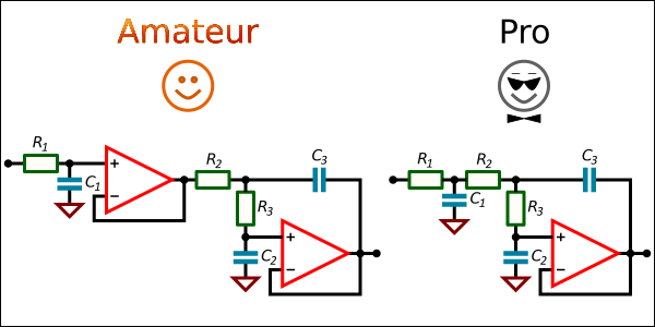
Common approach to build a 3rd order low-pass filter is to use two circuit stages and two Op Amps. Making a good One Op Amp design is not always easy, but it is possible.
Basic equations for third order low-pass filters
The transfer function of a 3rd order low-pass filter is:
                      A
H(s) = ———————————————————————————————
       (1 + s/ω₁)(1 + s/(Q ω₂) + s²/ω₂²)
where:
A – DC gain;
ω₁ – radial frequency of the first stage, K1 × ω;
ω₂ – radial frequency of the second stage, K2 × ω;
Q – quality factor of the second stage;
ω – pass-band radial frequency of the filter;
s – complex frequency.
Open brackets to have another form of the transfer function:
                   A                                 A                                 A
H(s) = ————————————————————————— = ————————————————————————————————————— = ———————————————————————————
       (1 + a s)(1 + b s + c s²)   1 + (a + b) s + (a b + c) s² + a c s³   1 + ps1 s + ps2 s² + ps3 s³

ps1 = 1 / ω₁ + 1 / (Q ω₂)
ps2 = 1 / (ω₁ Q ω₂) + 1/ω₂²
ps3 = 1 / (ω₁ ω₂²)
Knowing −3 dB frequency and filter type, we can get K1 and K2 from tables in books [1] or compute them to get ω1 and ω2.
Also, knowing ps1, ps2, ps3, the equations can be solved to find the filter radial frequencies and the quality factor. The solution is very long, therefore is omitted. You can find it using mathematical software.
Ways to build a third order low-pass filter
Standard approach to build multistage filters is to arrange stages from low to high quality factor stages. For 3rd order filters it means that the single pole filter stage is the first.
[2] says that it make sense to move the first-order stage at the end of the circuit to reduce the filter noise. This configuration can also avoid peaking due to high Q sections.
So, the easiest way to build a 3rd order low-pass filter with only one Op Amp is to add an RC circuit at the output of a second order filter. Unfortunately, if the filter must have low output impedance, this method cannot be used.
If we remove Op Amp from the first-order stage and connect an RC circuit to the second-order stage directly, the input impedance of the stage will affect RC circuit parameters. When it is high enough comparing with the R value, it can be done. Usually it is not the case, so the input impedance must be taken into account. Since it is frequency dependent, it is not so easy to compute filter component values.
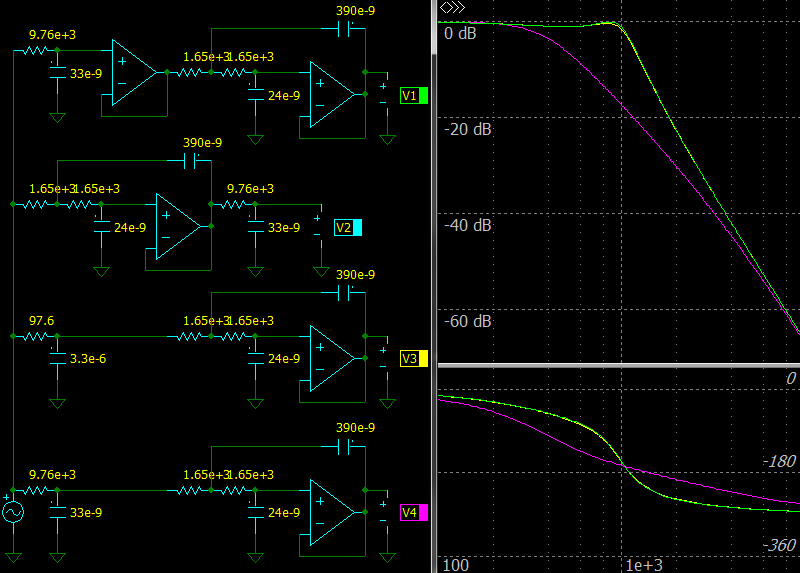 |
| 4 variants of a 3rd order Chebyshev low-pass filter using the Sallen-Key topology |
The picture above shows 4 variants of a 3rd order Chebyshev low-pass filter with the Sallen-Key topology. From top to bottom:
- The first circuit shows the standard way to design a third order low-pass filter, the green line in the chart.
- The second circuit shows that if the RC circuit is at the end, the frequency response is the same, the cyan line in the chart. The minimum resistor value is defined by minimum load of used Op Amp.
- The third circuit shows that if the R value of the RC circuit is low compared to the circuit input impedance, the frequency response is almost the same, the yellow line. The resistor value should be low, so a previous stage will have quite high load.
- The fourth circuit shows that if the first Op Amp is removed from the standard circuit and the RC values are the same, the frequency response changes dramatically, the purple line.
Third Order One Op Amp In-The-Loop Low-pass Filter
 |
| Third Order In-The-Loop Low-pass Filter |
Design Equations
This filter has active input impedance that is defined by its input resistance virtually connected to the ground and it is not hard to write its transfer function in the classic form assuming an ideal Op Amp:
                           − R3 / (R1 + R2)
H(s) = ——————————————————————————————————————————————————————————
       (1 + s C1 [R1 || R2])(1 + s C2 [R3 + R4] + C2 C3 R3 R4 s²)
So we can write that the radial cutoff frequencies are:
           1
ω1 = —————————————
     C1 (R1 || R2)

           1
ω2 = ——————————————
     √{C2 C3 R3 R4}
the quality factor is:
          √{C2 C3 R3 R4}
Q = ——————————————————————————
     C2 (R3 + R4 + R3 R4 / RL)
the DC gain is:
A = − R3 / (R1 + R2)
Example
Let’s compute the third order Butterworth filter with 150 kHz pass-band and unity gain.
For a 3rd order Butterworth filter
Choose the feedback R3 value, for example, 1 kOhm, and the R4 value, for example, 100 Ohm.
Now we can calculate the other component values, assuming that RL is high enough and may be ignored.
             1                              1
C2 = ———————————————— = ————————————————————————————————————————— ≈ 1 nF (E24)
     (R3 + R4) Q K2 ω   (1 Ohm + 100 Ohm) × 1 × 1 × 2 π × 150 kHz

     (R3 + R4) Q          (1 kOhm + 100 Ohm) × 1
C2 = ——————————— = ———————————————————————————————————— ≈ 12 nF (E24)
     R3 R4  K2 ω   1 kOhm × 100 Ohm × 1 × 2 π × 150 kHz

          R3   1 kOhm
R1 + R2 = —— = —————— = 1 kOhm (E96)
          A      1
Set
       R1 + R2               499 Ohm + 499 Ohm
C1 = —————————— = ——————————————————————————————————————— ≈ 4.3 nF (E24)
     R1 R2 K1 ω   (499 Ohm × 499 Ohm) × 1 × 2 π × 150 kHz
Use a simulator to verify our solution.
 |
| Third Order In-The-Loop Low-pass Filter, Frequency response |
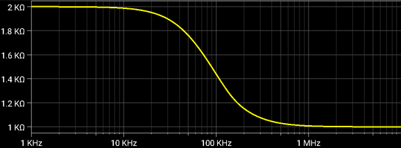
Magnitude of the input impedance is varying from (R1+R2) at low frequencies to the R1 value at high frequencies.
 |
| Third Order In-The-Loop Low-pass Filter, Input impedance |
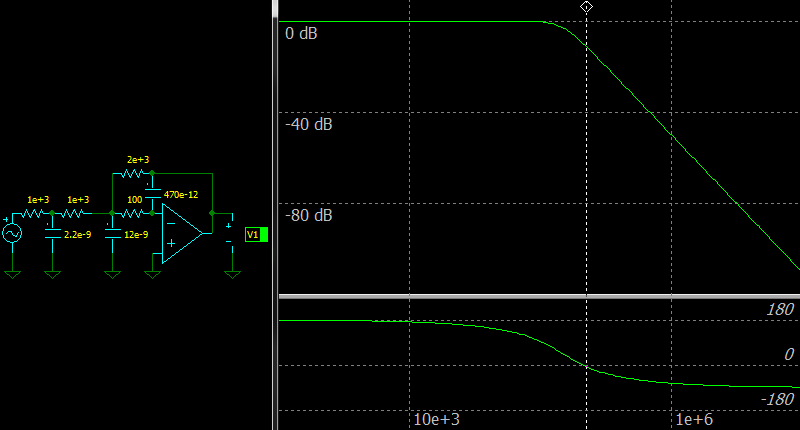
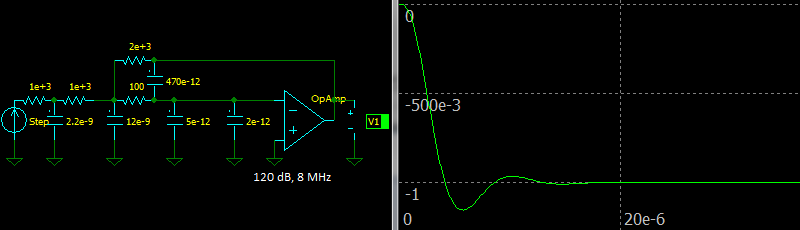
Let’s ensure that the circuit is stable and see step response of the circuit using parameters from the OPA2134 datasheet.
 |
| Third Order In-The-Loop Butterworth Low-pass Filter, Step response |
The step response is almost equal to the ideal filter step response which can be found in books.
A Fully Differential Amplifier can also be used, but the C1 and C3 values must be divided by 2.
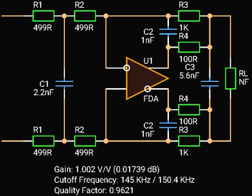 |
| Third Order In-The-Loop Low-pass Filter with Fully Differential Amplifier |
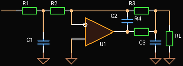
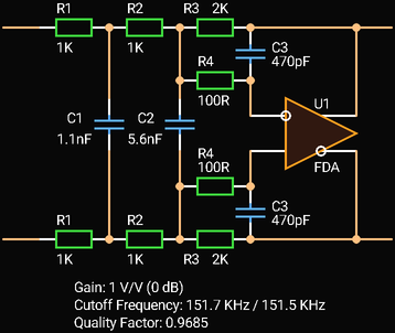
Third Order One Op Amp Multiple Feedback Low-pass Filter
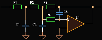 |
| Third Order Multiple Feedback Low-pass Filter |
Design Equations
The transfer function is:
                    A
H(s) = ———————————————————————————
       1 + ps1 s + ps2 s² + ps3 s³
Assuming an ideal Op Amp, the factors are:
      C1 R1 R2 + C3 [R3 R4 + (R1 + R2)(R3 + R4)]
ps1 = ——————————————————————————————————————————
                       R1 + R2

      C3 [C1 R1 (R3 R4 + R2 R3 + R2 R4) + C2 R3 R4 (R1 + R2)]
ps2 = ———————————————————————————————————————————————————————
                              R1 + R2

      C1 C2 C3 R1 R2 R3 R4
ps3 = ————————————————————
            R1 + R2
the DC gain is:
A = − R3 / (R1 + R2)
An analytical solution to get the filter parameters, if it even exists, is huge, so the only way to find a solution is to solve the equations numerically.
Example
Let’s compute the same 3rd order Butterworth filter with 150 kHz pass-band and unity gain.
Set
R3 = −A (R1 + R2) = −(−1) × (1 kOhm + 1 kOhm) = 2 kOhm (E96)

       1       1              1                     1
ps1 = ———— + —————— = ————————————————— + ————————————————————— ≈ 2.122e−6
      K1 ω   Q K2 ω   1 × 2 π × 150 kHz   1 × 1 × 2 π × 150 kHz

           1           1                          1                                1
ps2 = ——————————— + ——————— = ———————————————————————————————————————— + ———————————————————— ≈ 2.2516e−12
      K1 ω Q K2 ω   (K2 ω)²   1 × 2 π× 150 kHz × 1 × 1 × 2 π × 150 kHz   (1 × 2 π × 150 kHz)²

            1                           1
ps3 = ———————————— = ———————————————————————————————————————— ≈ 1.195e−18
      K1 ω (K2 ω)²   1 × 2 π × 150 kHz × (1 × 2 π × 150 kHz)²
There are 3 equations and 4 unknown values: C1, C2, C3, R4.
Analysis shows that the equations have solutions for C1, C2, C3 at any R4 values. C2 cannot be too low, C3 cannot be too big, and C1 defines R1, R2, R3 too. It shows also that there is no solution with
So, the only appropriate way to find a solution is to set an R4 value and solve the equations to find C1, C2, C3.
Let’s set
The solution is:
Simulation confirms that our solution is correct.
 |
| Third Order Multiple Feedback Low-pass Filter, Frequency response |
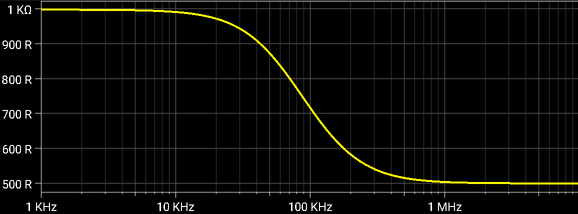
Magnitude of the input impedance is varying from (R1+R2) at low frequencies to the R1 value at high frequencies.
 |
| Third Order Multiple Feedback Low-pass Filter, Input impedance |
Let’s ensure that the circuit is stable and see step response of the circuit using parameters from the OPA2134 datasheet.
 |
| Third Order Multiple Feedback Butterworth Low-pass Filter, Step response |
A Fully Differential Amplifier can also be used, but the C1 and C2 values must be divided by 2.
 |
| Third Order Multiple Feedback Low-pass Filter with Fully Differential Amplifier |
Third Order One Op Amp Sallen-Key Low-pass Filter
 |
| Third Order Sallen-Key Low-pass Filter |
Design Equations
The transfer function is:
                    A
H(s) = ———————————————————————————
       1 + ps1 s + ps2 s² + ps3 s³
Assuming an ideal Op Amp, the factors are:
ps1 = C1 R1 + C2 (R1 + R2 + R3) − C3 (R1 + R2) R5 / R4

ps2 = C1 R1 (C2 (R2 + R3) − C3 R2 R5 / R4) + C2 C3 R3 (R1 + R2)

ps3 = C1 C2 C3 R1 R2 R3
the DC gain is:
A = 1 + R5 / R4
Example
Let’s compute the same 3rd order Butterworth filter with 150 kHz pass-band and unity gain.
For unity gain: R5 = 0, R4 is not installed.
The factor values are already known:
ps1 ≈ 2.122e−6
ps2 ≈ 2.2516e−12
ps3 ≈ 1.195e−18
There are 3 equations and 6 unknown values: C1, C2, C3, R1, R2, R3.
Usually engineers want to optimize bill of materials, so solutions with
Solutions with
Set
Simulation confirms that our solution is right.
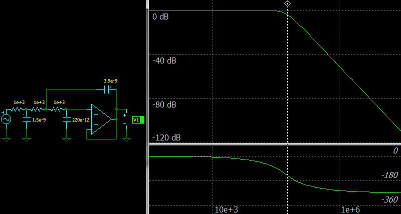 |
| Third Order Sallen-Key Low-pass Filter, Frequency response |
Magnitude of the input impedance is varying from a very high value at low frequencies to the R1 value at high frequencies.
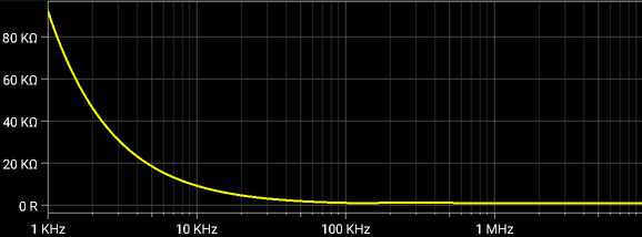 |
| Third Order Sallen-Key Low-pass Filter, Input impedance |
Let’s ensure that the circuit is stable and see step response of the circuit using parameters from the OPA2134 datasheet.
 |
| Third Order Sallen-Key Butterworth Low-pass Filter, Step response |
The step response is similar to the ideal filter step response. There is no oscillation, so the circuit can be used.
Conclusion
There are several ways to build a 3rd order low-pass filter using only one Op Amp:
- Add an RC circuit at the end of a second order stage. The advantage is reducing noise and peaking. The disadvantage is increasing output impedance.
- Add an RC circuit at the front of the second order stage ignoring its input impedance. It works only if the R value is much lower than the input impedance of the second stage or if the impedance is constant over the frequency range and can be taken into account, like in the In-The-Loop Low-pass Filter.
- Add an RC circuit at the front of the second order stage and solve equations to find appropriate component values.
Knowing a solution for some case, it is possible to scale component values to find other solutions to avoid solving the equations from scratch. This way is used in some online tools. But if you want to optimize your bill of materials and minimize tolerances, you have to solve the equations varying initial values to find the best component values.
References
- Analog Devices. “Linear Circuit Design Handbook”. Chapter 8, “Analog Filters”.
- Bonnie Baker, “Painless reduction of analog filter noise”.
- L.K. Wadhwa, “One Operational Amplifier Simulates Third Order Systems with Double lead”.
- Christopher Paul, “Design second- and third-order Sallen-Key filters with one op amp”.
- Christopher Paul, “Building optimal sensitivity third order low pass filters with a single op amp”.
- Christopher Paul, “A Sallen-Key low-pass filter design toolkit”.
- OKAWA Electronic Design, “3rd order Sallen-Key Low-pass Filter Design Tool”.
- The Electronics Section of Beis.de, “Dimensioning of Active 3-Pole Single Stage Low-Pass Filters”.
- Active filter design software “Aktiv Filter”.
- Nuhertz Technologies, Active Filter Module.
- «idealCircuit», a simulator.
- «Filter Designer», a multistage analog active filter design tool for Android
- «Circuit Calculator», an electronics circuit design tool for Android.
