Photo by Dugan Arnett on Boston Globe
Are you still looking for a new flat? Ready to make the last attempt? If so - follow me and I show you how to reach the finish line.
Short introduction and references
It is the third part of the cycle directed to explain how could you find the optimal flat on the real estate market. In a few words the main idea - find the best offer among apartments in Yekaterinburg, where I lived before. But I think the same idea can be considered in the context of another city.
If you have not read the previous parts, it would be a good idea to read them Part1 and Part2.
Also, you could find out Ipython-notebooks over there.
This part had to be much shorter than previous ones, but the devil is in details.
Consequences
As a result of all actions, we got an ML model (Random Forest) which works quite well. Not so good as we expected (the score is above 87%), but for real data, it is good enough. And… let me be honest, that thoughts about result had a strange affect on me. I wanted more score, the gap between the result which was expected and the real prediction was smaller than 3%. Optimism mixed with greed has gone to my head

I want more gold accuracy
It is widely known, if you want to improve something there will be probably opposite approaches. Usually, it looks like a choice between:
- Evolution vs revolution
- Quantity vs quality
- Extensive vs intensive
And because of a lack of will to change horses in midstream, I decided to use RF (Random Forest) with adding a few new features.
It seemed like an idea, "we just need more features" for making the score better. At least that is what I thought.
Per aspera ad astra (through hardships to the stars)
Let's try to think about related features, which could influence a flat's price. There are features of flat like balcony or age of house and geo-related features like distance to the nearest metro/bus station. What could be next for the same approach with RF?
Idea #1. Distance to centre
We could reuse longitude and latitude (flat coordinates). Base on this information we could count the distance to the centre of the city. The same idea was used for districts, the far we flat located from the centre, the cheaper it should be. And guess what… it works! Not such big growth (+1% of score), but it is better than nothing.
Only one problem is there, the same idea does not make sense for districts which are very far. If you lived outside a city, you could know that there are other rules for the price.
It will not be easy for interpretation if we extrapolate that approach.
Idea #2. Near metro
The metro has a significant influence on price. Especially when it placed in a zone of walking distance. But the meaning of "a walking distance" is not clear. Each person can interpret that parameter in different ways. I could set the limit by manually, but an increase of score would not be over 0.2%
At the same time, it does not work with flat from the previous idea. There is no metro nearby.
Idea #3. Rationality and equilibrium of the market
The equilibrium of the market is a combination of demand and offer. Adam Smith talked about it. Of course, the market can be overblown. But in general, this idea works well. At least for houses which in the process of construction.
In other words - the more competitors do you have the less probability that people buy your flat (other things being equal). And this produces a supposition - "if around me are placed other flats I need to decrease the price for getting more buyers".
And It sounds like a quite logical conclusion, is not it?
So I counted SIMILAR flats near each of them, in the same house and within radius 200 meters. The measures were made for date of selling. Which result would you expect to take? Only 0.1% on cross-validation. Sad but true.
Rethinking
Quitting Is … sometimes to take one step backward to take two steps forward.
— an unknown wise person
Okay, a head-on attack does not work. Let's consider this situation from another angle.
Let suppose you are a person who wants to buy a flat near-by river far from the noisy city. You have three variants of advertisement which are similar to each other and price the same (more or less). Formal metrics which describing flat gives you nothing about the environment, they are only metrics on a screen. But there is something important.
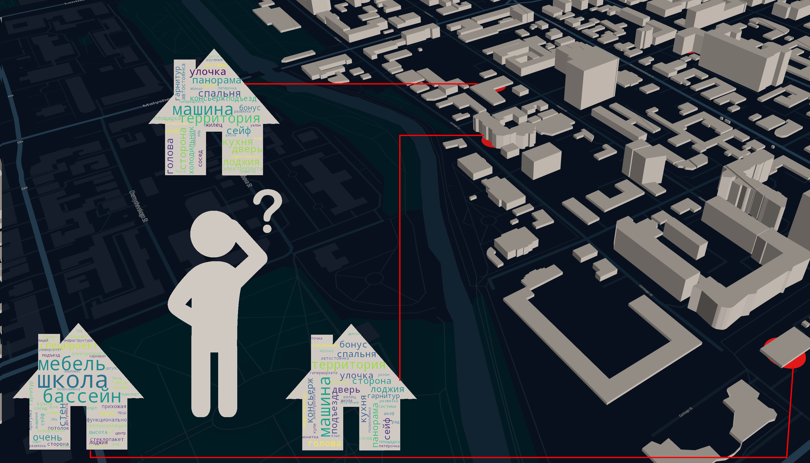
A description of a flat is a terrific opportunity.
A flat description could provide everything that you need. It could tell you a story about flat, about neighbours and amazing opportunities related to that specific living place. And sometime one description could make more sense than boring numbers.
But in real life is slightly different from our expectation. Let me show you what will/will not work and why.
What will not work and why?
Expectations - "Whoa! I can try to classify text and find 'good' and 'bad' flats. I will use the same method which usually used for sentiment analyse".
Reality - "No, you will not do it. People write nothing bad against their flat. There can be glossing over a real situation or lie"
Expectations - "Okay. Then I can try to find patterns and find the target audience for a flat. For instance, it could be elderly people or students".
Reality - "No, you will not do it. Sometimes one advertisement has a mention about different ages and social groups, it is just marketing"
What probably would work and why
Some keywords - There are words which point out at specific things or moments related to flat. For example, when it is a studio, price would be lower. In general, verbs are useless, but nouns and adverbs can give more context.
The alternative source of information - Using description for filling empty or NaN-values more correct. Sometimes the description contains more information than formal features of advertisement.
I suspect it based on human laziness to fill not required fields like "balcony". Putting everything in the description seems like a more preferable idea
Getting information
I skip describing of the typical process of tokenisation/lemmatization/stemming. Also, I believe that there are authors able to describe it better than me.
Although I think there should be a mention of the toolset used for extracting features. In nutshell, it looks like.

separating->matching by part of speech
After pre-processing of advertisement text I got a set of Russian words like these.

The original text is placed https://pastebin.com/Pxh8zVe3
I tried to use the approach from Word2Vec, but there was not a special dictionary for flats and advertisements, so the general picture looked weird
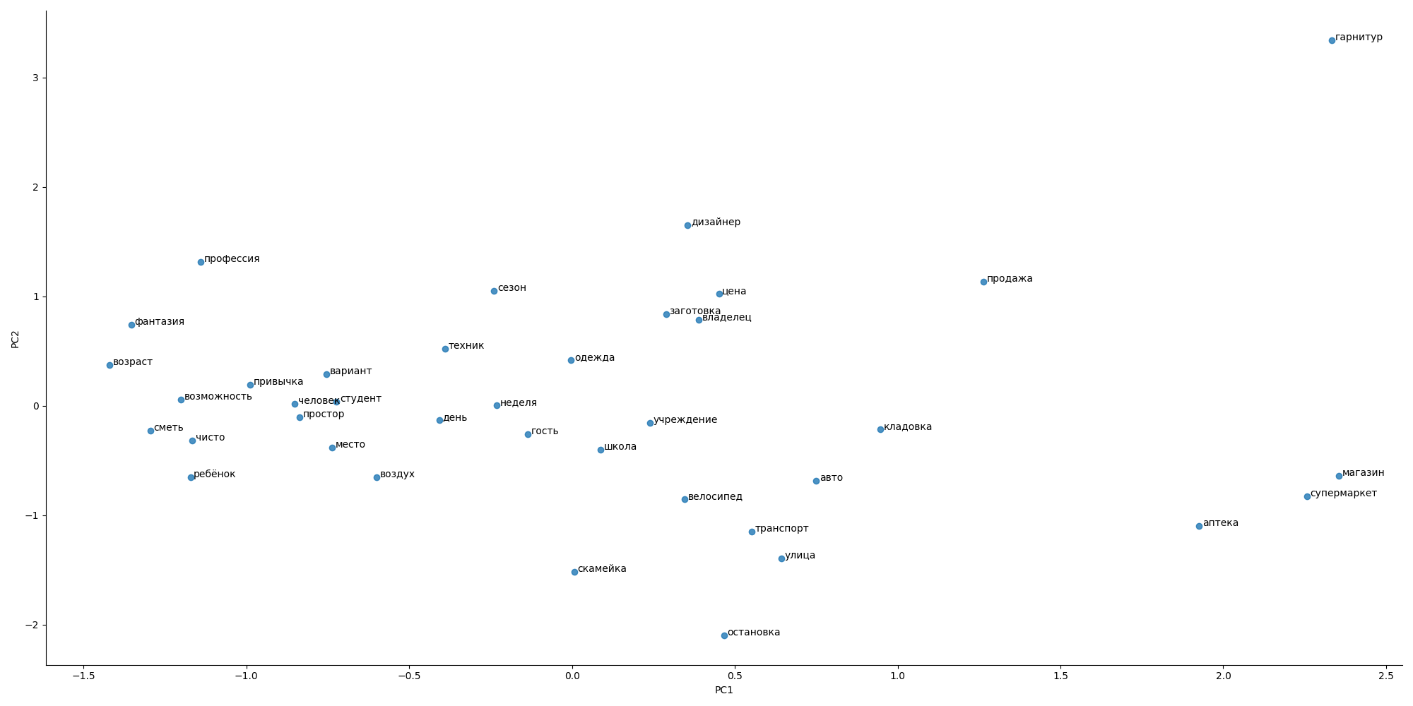
the distance between words does not suitable to expectations
Therefore I kept it as simple as possible and decided to make several new columns for dataset
A little less conversation, a little more action
Time to get our hands dirty and do some practical things. Find out new features. Several important factors were separated by an influence on price.
positive impact
- furniture — sometimes people could leave a bed, a washer and so on.
- luxury - flats with luxurious things like jacuzzi, or an exclusive interior
- video-control - it makes people feel safe, frequently it considers it as advantage
negative impact
- dorm - yes, sometimes it is a flat in a dorm. Not s o popular, but significantly cheaper than an average flat
- rush - when people rush to sell out their flat usually they are ready to decrease price.
- studio - as I said before - they are cheaper than their flats-analogues.
Let's collect them in something universal
df3 = pd.read_csv('flats3.csv')

positive_impact = ['мебель', 'luxury','видеонаблюдение']
negative_impact  = ['studio', 'rush','dorm']
geo_features = ['metro','num_of_stops_1km','num_of_shops_1km','num_of_kindergarden_1km',          'num_of_medical_1km','center_distance']
flat_features=['total_area', 'repair','balcony_y', 'walls_y','district_y', 'age_y']
competitors_features = ['distance_200m', 'same_house']
cols = ['cost']
cols+=flat_features
cols+=geo_features
cols+=competitors_features
cols+=positive_impact
cols+=negative_impact
df3 = df3[cols]
general impact
it is just a combination of negative and positive features. Initially, for every flat, it equals 0. For example, studio with video-control will still have general impact equals 0(1[positive]–1[negative]=0)
df3['impact'] = 0
for i, row in df3.iterrows():
    impact = 0
    for positive in  positive_impact:
        if row[positive]:
             impact+=1
    for negative in  negative_impact:
        if row[negative]:
            impact-=1
    df3.at[i, 'impact'] = impact
Okay, we have a data, new features and old target with 10% of mean error for prediction. Do some typical operation as we did before
y = df3.cost
X = df3.drop(columns=['cost'])

X_train, X_test, y_train, y_test = train_test_split(X, y, test_size=0.2,                                                random_state=42)
Old approach(extensive growth of features)
We will make a new model based on old ideas
data = []
max_features =  int(X.shape[1]/2)
for x in range(1,20):
    regressor = RandomForestRegressor(verbose=0,
                                      n_estimators=128,
                                      max_features=max_features,
                                      max_depth=x,
                                      random_state=42)
    model =   regressor.fit(X_train, y_train)
    score = do_cross_validation(X, y, model)
    data.append({'max_depth':x,'score':score})
data = pd.DataFrame(data)
f, ax = plot.subplots(figsize=(10, 10))
sns.lineplot(x="max_depth", y="score", data=data)
max_result = data.loc[data['score'].idxmax()]

ax.set_title(f'Max score - {max_result.score}\nDepth {max_result.max_depth} ')
And the result was slightly… unexpected.
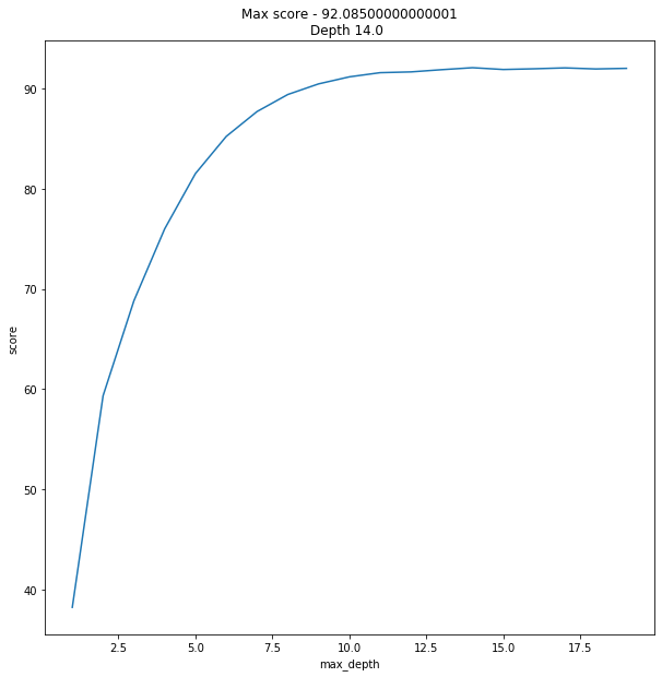
92% is overwhelming result. I mean, to say I was shocked would be an understatement.
But why it worked so well? Let's have a look at new features.
regressor = RandomForestRegressor(random_state=42,
                                  max_depth=max_result.max_depth,
                                  n_estimators=128,
                                  max_features=max_features)
rf3 =   regressor.fit(X_train, y_train)
feat_importances = pd.Series(rf3.feature_importances_, index=X.columns)
feat_importances.nlargest(X.shape[1]).plot(kind='barh')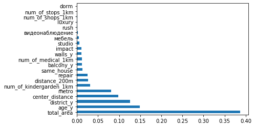
Importance all features for our model
The importance does not give information about the contribution of features(that is a different story ), it is only showing how active model use one or another feature. But for the current situation, it looks informative. Some of the new features are more important than previous ones, others almost useless.
New approach(intensive work with data)
Well… the finish line is crossed, the result is achieved. Could it be better?
Short answer - "Yes, it could"
- First, we could reduce the depth of a tree. It will lead to a smaller time for training and prediction as well.
- Second, we could a little bit increase a score of prediction.
For both moments we will use XGBoost. Sometimes people prefer to use other boosters like LightGBM or CatBoost, but my humble opinion - the first one is good enough when you have a lot of data, a second one is better if you have work with categorical variables. And as a bonus - XGBoost just seems faster
from xgboost import XGBRegressor,plot_importance
data = []
for x in range(3,10):
    regressor = XGBRegressor(verbose=0,
                             reg_lambda=10,
                             n_estimators=1000,
                             objective='reg:squarederror',
                             max_depth=x,
                             random_state=42)

    model =   regressor.fit(X_train, y_train)
    score = do_cross_validation(X, y, model)
    data.append({'max_depth':x,'score':score})
data = pd.DataFrame(data)
f, ax = plot.subplots(figsize=(10, 10))
sns.lineplot(x="max_depth", y="score", data=data)
max_result = data.loc[data['score'].idxmax()]

ax.set_title(f'Max score-{max_result.score}\nDepth {max_result.max_depth} ')
The result is better than the previous one.
Of course, it is the not big difference between Random Forest and XGBoost. And each of them could be used as a good tool for resolving our problem with prediction. It is up to you.
Conclusion
Is the result achieved? Definitely yes.
The solution is available there and can be used anyone for free. If you are interested in the evaluation of an apartment using this approach, please do not hesitate and contact me.
As prototype it placed there
Thank you for reading!.
