In the previous articles, we discussed PostgreSQL indexing engine, the interface of access methods, and two access methods: hash index and B-tree. In this article, we will describe GiST indexes.
GiST is an abbreviation of «generalized search tree». This is a balanced search tree, just like «b-tree» discussed earlier.
What is the difference? «btree» index is strictly connected to the comparison semantics: support of «greater», «less», and «equal» operators is all it is capable of (but very capable!) However, modern databases store data types for which these operators just make no sense: geodata, text documents, images,…
GiST index method comes to our aid for these data types. It permits defining a rule to distribute data of an arbitrary type across a balanced tree and a method to use this representation for access by some operator. For example, GiST index can «accommodate» R-tree for spatial data with support of relative position operators (located on the left, on the right, contains, etc.) or RD-tree for sets with support of intersection or inclusion operators.
Thanks to extensibility, a totally new method can be created from scratch in PostgreSQL: to this end, an interface with the indexing engine must be implemented. But this requires premeditation of not only the indexing logic, but also mapping data structures to pages, efficient implementation of locks, and support of a write-ahead log. All this assumes high developer skills and a large human effort. GiST simplifies the task by taking over low-level problems and offering its own interface: several functions pertaining not to techniques, but to the application domain. In this sense, we can regard GiST as a framework for building new access methods.
GiST is a height-balanced tree that consists of node pages. The nodes consist of index rows.
Each row of a leaf node (leaf row), in general, contains some predicate (boolean expression) and a reference to a table row (TID). Indexed data (key) must meet this predicate.
Each row of an internal node (internal row) also contains a predicate and a reference to a child node, and all indexed data of the child subtree must meet this predicate. In other words, the predicate of an internal row comprises the predicates of all child rows. This important trait of GiST index replaces simple ordering of B-tree.
Search in GiST tree uses a specialized consistency function («consistent») — one of the functions defined by the interface and implemented in its own way for each supported operator family.
The consistency function is called for an index row and determines whether the predicate of this row is consistent with the search predicate (specified as "indexed-field operator expression"). For an internal row, this function actually determines whether it is needed to descend to the corresponding subtree, and for a leaf row, the function determines whether the indexed data meets the predicate.
The search starts with a root node, as a normal tree search. The consistency function permits to find out which child nodes it makes sense to enter (there may be several of them) and which it does not. The algorithm is then repeated for each child node found. And if the node is leaf, the row selected by the consistency function is returned as one of the results.
The search is depth-first: the algorithm first tries to reach a leaf node. This permits to return first results soon whenever possible (which might be important if the user is interested in only several results rather than all of them).
Let's once again note that the consistency function does not need to have anything to do with «greater», «less», or «equal» operators. The semantics of the consistency function may be quite different and therefore, the index is not assumed to return values in a certain order.
We will not discuss algorithms of insertion and deletion of values in GiST: a few more interface functions perform these operations. There is one important point however. When a new value is inserted into the index, the position for this value in the tree is selected so that the predicates of its parent rows are extended as little as possible (ideally, not extended at all). But when a value is deleted, the predicate of the parent row is not reduced anymore. This only happens in cases like these: a page is split into two ones (when the page does not have enough space for insertion of a new index row) or the index is recreated from scratch (with REINDEX or VACUUM FULL command). Therefore, efficiency of GiST index for frequently changing data can degrade over time.
Further we will consider a few examples of indexes for various data types and useful properties of GiST:
We will illustrate the above by example of an index for points in a plane (we can also build similar indexes for other geometric entities). A regular B-tree does not suit this data type of data since no comparison operators are defined for points.
The idea of R-tree is to split the plane into rectangles that in total cover all the points being indexed. An index row stores a rectangle, and the predicate can be defined like this: «the point sought lies within the given rectangle».
The root of the R-tree will contain several largest rectangles (possibly intersecting). Child nodes will contain smaller-size rectangles that are embedded in the parent one and in total cover all underlying points.
In theory, leaf nodes must contain points being indexed, but the data type must be the same in all index rows and therefore, again rectangles are stored, but «collapsed» into points.
To visualize such a structure, we provide images for three levels of the R-tree. Points are coordinates of airports (similar to those from the «airports» table of the demo database, but more data from openflights.org is provided).

Level one: two large intersecting rectangles are visible.

Level two: large rectangles are split into smaller areas.

Level three: each rectangle contains as many points as to fit one index page.
Now let's consider a very simple «one-level» example:

With this splitting, the index structure will look as follows:

The index created can be used to speed up the following query, for example: «find all points contained in the given rectangle». This condition can be formalized as follows:
The consistency function of the operator ("indexed-field <@ expression", where indexed-field is a point and expression is a rectangle) is defined as follows. For an internal row, it returns «yes» if its rectangle intersects with the rectangle defined by the expression. For a leaf row, the function returns «yes» if its point («collapsed» rectangle) is contained in the rectangle defined by the expression.
The search starts with the root node. The rectangle (2,1)-(7,4) intersects with (1,1)-(6,3), but does not intersect with (5,5)-(8,8), therefore, there is no need to descend to the second subtree.

Upon reaching a leaf node, we go through the three points contained there and return two of them as the result: (3,2) и (6,3).
Unfortunately, customary «pageinspect» does not allow looking into GiST index. But another way is available: «gevel» extension. It is not included in the standard delivery, so see the installation instructions.
If all is done right, three functions will be available to you. First, we can get some statistics:
It is clear that the size of the index on airport coordinates is 690 pages and that the index consists of four levels: the root and two internal levels were shown in figures above, and the fourth level is leaf.
Actually, the index for eight thousand points will be considerably smaller: here it was created with a 10% fillfactor for clarity.
Second, we can output the index tree:
And third, we can output the data stored in index rows. Note the following nuance: the result of the function must be cast to the data type needed. In our situation, this type is «box» (a bounding rectangle). For example, notice five rows at the top level:
Actually, the figures provided above were created just from this data.
Operators discussed so far (such as
There is also another operator type: ordering operators. They are used for specifications of the sort order in ORDER BY clause instead of conventional specifications of column names. The following is an example of such a query:
To support queries of this kind, an access method must define an additional distance function, and the ordering operator must be included in the appropriate operator class (for example, «points_ops» class for points). The query below shows operators, along with their types («s» — search and «o» — ordering):
The numbers of strategies are also shown, with their meanings explained. It is clear that there are far more strategies than for «btree», only some of them being supported for points. Different strategies can be defined for other data types.
The distance function is called for an index element, and it must compute the distance (taking into account the operator semantics) from the value defined by the expression ("indexed-field ordering-operator expression") to the given element. For a leaf element, this is just the distance to the indexed value. For an internal element, the function must return the minimum of the distances to the child leaf elements. Since going through all child rows would be pretty costly, the function is permitted to optimistically underestimate the distance, but at the expense of reducing the search efficiency. However, the function is never permitted to overestimate the distance since this will disrupt the work of the index.
The distance function can return values of any sortable type (to order values, PostgreSQL will use comparison semantics from the appropriate operator family of «btree» access method, as described earlier).
For points in a plane, the distance is interpreted in a very usual sense: the value of
Let's consider the search algorithm for the above query.
The search starts with the root node. The node contains two bounding rectangles. The distance to (1,1)-(6,3) is 4.0 and to (5,5)-(8,8) is 1.0.
Child nodes are walked through in the order of increasing the distance. This way, we first descend to the nearest child node and compute the distances to the points (we will show the numbers in the figure for visibility):
This information suffices to return the first two points, (5,5) and (7,8). Since we are aware that the distance to points that lie within the rectangle (1,1)-(6,3) is 4.0 or greater, we do not need to descend to the first child node.
But what if we needed to find the first three points?
Although the second child node contains all these points, we cannot return (8,6) without looking into the first child node since this node can contain closer points (since 4.0 < 4.1).

For internal rows, this example clarifies requirements for the distance function. By selecting smaller distance (4.0 instead of actual 4.5) for the second row, we reduced the efficiency (the algorithm needlessly started examining an extra node), but did not break correctness of the algorithm.
Until recently, GiST was the only access method capable of dealing with ordering operators. But the situation has changed: RUM access method (to be discussed further) has already joined this group of methods, and it is not unlikely that good old B-tree will join them: a patch developed by Nikita Glukhov, our colleague, is being discussed by the community.
Another example of using GiST access method is indexing of intervals, for example, time intervals («tsrange» type). All the difference is that internal nodes will contain bounding intervals instead of bounding rectangles.
Let's consider a simple example. We will be renting out a cottage and storing reservation intervals in a table:
The index can be used to speed up the following query, for example:
Note that this is either not about getting intervals in a certain order, although comparison operators are defined for intervals. We can use «btree» index for intervals, but in this case, we will have to do without support of operations like these:
(Except the equality, which is contained in the operator class for «btree» access method.)
We can look inside using the same «gevel» extension. We only need to remember to change the data type in the call to gist_print:
GiST index can be used to support exclusion constraints (EXCLUDE).
The exclusion constraint ensures given fields of any two table rows not to «correspond» to each other in terms of some operators. If «equals» operator is chosen, we exactly get the unique constraint: given fields of any two rows do not equal each other.
The exclusion constraint is supported by the index, as well as the unique constraint. We can choose any operator so that:
This is a list of suitable strategies and examples of operators (operators, as we remember, can have different names and be available not for all data types):
Note that we can use the equality operator in an exclusion constraint, but it is impractical: a unique constraint will be more efficient. That is exactly why we did not touch upon exclusion constraints when we discussed B-trees.
Let's provide an example of using an exclusion constraint. It is reasonable not to permit reservations for intersecting intervals.
Once we created the exclusion constraint, we can add rows:
But an attempt to insert an intersecting interval into the table will result in an error:
Let's complicate the problem. We expand our humble business, and we are going to rent out several cottages:
We need to change the exclusion constraint so that house numbers are taken into account. GiST, however, does not support the equality operation for integer numbers:
In this case, "btree_gist" extension will help, which adds GiST support of operations inherent to B-trees. GiST, eventually, can support any operators, so why should not we teach it to support «greater», «less», and «equal» operators?
Now we still cannot reserve the first cottage for the same dates:
However, we can reserve the second one:
But be aware that although GiST can somehow support «greater», «less», and «equal» operators, B-tree still does this better. So it is worth using this technique only if GiST index is essentially needed, like in our example.
Let's start with a minimalist introduction to PostgreSQL full-text search (if you are in the know, you can skip this section).
The task of full-text search is to select from the document set those documents that match the search query. (If there are many matching documents, it is important to find the best matching, but we will say nothing about it at this point.)
For search purposes, a document is converted to a specialized type «tsvector», which contains lexemes and their positions in the document. Lexemes are words converted to the form suitable for search. For example, words are typically converted to lowercase, and variable endings are cut off:
We can also see that some words (called stop words) are totally dropped («there», «was», «a», «and», «he») since they presumably occur too often for search of them to make sense. All these conversions can certainly be configured, but that's another story.
A search query is represented with another type: «tsquery». Roughly, a query consists of one or several lexemes joint by connectives: «and» &, «or» |, «not»!.. We can also use parentheses to clarify operation precedence.
Only one match operator
This information suffices for now. We will dive a little deeper into full-text search in a next article that features GIN index.
For fast full-text search, firstly, the table needs to store a column of type «tsvector» (to avoid performing a costly conversion each time when searching) and secondly, an index must be built on this column. One of possible access methods for this is GiST.
It is, certainly, convenient to entrust a trigger with the last step (conversion of the document to «tsvector»).
How should the index be structured? Use of R-tree directly is not an option since it is unclear how to define a «bounding rectangle» for documents. But we can apply some modification of this approach for sets, a so-called RD-tree (RD stands for «Russian Doll»). A set is understood to be a set of lexemes in this case, but in general, a set can be any.
An idea of RD-trees is to replace a bounding rectangle with a bounding set, that is, a set that contains all elements of child sets.
An important question arises how to represent sets in index rows. The most straightforward way is just to enumerate all elements of the set. This might look as follows:

Then for example, for access by condition

This representation has evident issues. The number of lexemes in a document can be pretty large, so index rows will have large size and get into TOAST, making the index far less efficient. Even if each document has few unique lexemes, the union of sets may still be very large: the higher to the root the larger index rows.
A representation like this is sometimes used, but for other data types. And full-text search uses another, more compact, solution — a so-called signature tree. Its idea is quite familiar to all who dealt with Bloom filter.
Each lexeme can be represented with its signature: a bit string of a certain length where all bits but one are zero. The position of this bit is determined by the value of hash function of the lexeme (we discussed internals of hash functions earlier).
The document signature is the bitwise OR of the signatures of all document lexemes.
Let's assume the following signatures of lexemes:
Then signatures of the documents are like these:
The index tree can be represented as follows:
The advantages of this approach are evident: index rows have equal small sizes, and such an index is compact. But a drawback is also clear: the accuracy is sacrificed to compactness.
Let's consider the same condition
Compare with the figure above: we can see that the tree turned yellow, which means that false positives occur and excessive nodes are went through during the search. Here we picked up «whoever» lexeme, whose signature unfortunately was the same as the signature of «sit» lexeme. It's important that no false negatives can occur in the pattern, that is, we are sure not to miss needed values.
Besides, it may so happen that different documents will also get the same signatures: in our example, unlucky documents are «I slit a sheet, a sheet I slit» and «I slit sheets» (both have the signature of 0001100). And if a leaf index row does not store the value of «tsvector», the index itself will give false positives. Of course, in this case, the method will ask the indexing engine to recheck the result with the table, so the user will not see these false positives. But the search efficiency may get compromised.
Actually, a signature is 124-byte large in the current implementation instead of 7-bit in the figures, so the above issues are much less likely to occur than in the example. But in reality, much more documents get indexed as well. To somehow reduce the number of false positives of the index method, the implementation gets a little tricky: the indexed «tsvector» is stored in a leaf index row, but only if its size is not large (a little less than 1/16 of a page, which is about half a kilobyte for 8-KB pages).
To see how indexing works on actual data, let's take the archive of «pgsql-hackers» email. The version used in the example contains 356125 messages with the send date, subject, author, and text:
Adding and filling in the column of «tsvector» type and building the index. Here we will join three values in one vector (subject, author, and message text) to show that the document does not need to be one field, but can consist of totally different arbitrary parts.
As we can see, a certain number of words were dropped because of too large size. But the index is eventually created and can support search queries:
We can see that together with 898 rows matching the condition, the access method returned 7859 more rows that were filtered out by rechecking with the table. This demonstrates a negative impact of the loss of accuracy on the efficiency.
To analyze the contents of the index, we will again use «gevel» extension:
Values of the specialized type «gtsvector» that are stored in index rows are actually the signature plus, maybe, the source «tsvector». If the vector is available, the output contains the number of lexemes (unique words), otherwise, the number of true and false bits in the signature.
It is clear that in the root node, the signature degenerated to «all ones», that is, one index level became absolutely useless (and one more became almost useless, with only four false bits).
Let's look at the properties of GiST access method (queries were provided earlier):
Sorting of values and unique constraint are not supported. As we've seen, the index can be built on several columns and used in exclusion constraints.
The following index-layer properties are available:
And the most interesting properties are those of the column layer. Some of the properties are independent of operator classes:
(Sorting is not supported; the index cannot be used to search an array; NULLs are supported.)
But the two remaining properties, «distance_orderable» and «returnable», will depend on the operator class used. For example, for points we will get:
The first property tells that the distance operator is available for search of nearest neighbors. And the second one tells that the index can be used for index-only scan. Although leaf index rows store rectangles rather than points, the access method can return what's needed.
The following are the properties for intervals:
For intervals, the distance function is not defined and therefore, search of nearest neighbors is not possible.
And for full-text search, we get:
Support of index-only scan has been lost since leaf rows can contain only the signature without the data itself. However, this is a minor loss since nobody is interested in the value of type «tsvector» anyway: this value is used to select rows, while it is source text that needs to be shown, but is missing from the index anyway.
Finally, we will mention a few more types that are currently supported by GiST access method in addition to already discussed geometric types (by example of points), intervals, and full-text search types.
Of standard types, this is the type "inet" for IP-addresses. All the rest is added through extensions:
Read on.
GiST
GiST is an abbreviation of «generalized search tree». This is a balanced search tree, just like «b-tree» discussed earlier.
What is the difference? «btree» index is strictly connected to the comparison semantics: support of «greater», «less», and «equal» operators is all it is capable of (but very capable!) However, modern databases store data types for which these operators just make no sense: geodata, text documents, images,…
GiST index method comes to our aid for these data types. It permits defining a rule to distribute data of an arbitrary type across a balanced tree and a method to use this representation for access by some operator. For example, GiST index can «accommodate» R-tree for spatial data with support of relative position operators (located on the left, on the right, contains, etc.) or RD-tree for sets with support of intersection or inclusion operators.
Thanks to extensibility, a totally new method can be created from scratch in PostgreSQL: to this end, an interface with the indexing engine must be implemented. But this requires premeditation of not only the indexing logic, but also mapping data structures to pages, efficient implementation of locks, and support of a write-ahead log. All this assumes high developer skills and a large human effort. GiST simplifies the task by taking over low-level problems and offering its own interface: several functions pertaining not to techniques, but to the application domain. In this sense, we can regard GiST as a framework for building new access methods.
Structure
GiST is a height-balanced tree that consists of node pages. The nodes consist of index rows.
Each row of a leaf node (leaf row), in general, contains some predicate (boolean expression) and a reference to a table row (TID). Indexed data (key) must meet this predicate.
Each row of an internal node (internal row) also contains a predicate and a reference to a child node, and all indexed data of the child subtree must meet this predicate. In other words, the predicate of an internal row comprises the predicates of all child rows. This important trait of GiST index replaces simple ordering of B-tree.
Search in GiST tree uses a specialized consistency function («consistent») — one of the functions defined by the interface and implemented in its own way for each supported operator family.
The consistency function is called for an index row and determines whether the predicate of this row is consistent with the search predicate (specified as "indexed-field operator expression"). For an internal row, this function actually determines whether it is needed to descend to the corresponding subtree, and for a leaf row, the function determines whether the indexed data meets the predicate.
The search starts with a root node, as a normal tree search. The consistency function permits to find out which child nodes it makes sense to enter (there may be several of them) and which it does not. The algorithm is then repeated for each child node found. And if the node is leaf, the row selected by the consistency function is returned as one of the results.
The search is depth-first: the algorithm first tries to reach a leaf node. This permits to return first results soon whenever possible (which might be important if the user is interested in only several results rather than all of them).
Let's once again note that the consistency function does not need to have anything to do with «greater», «less», or «equal» operators. The semantics of the consistency function may be quite different and therefore, the index is not assumed to return values in a certain order.
We will not discuss algorithms of insertion and deletion of values in GiST: a few more interface functions perform these operations. There is one important point however. When a new value is inserted into the index, the position for this value in the tree is selected so that the predicates of its parent rows are extended as little as possible (ideally, not extended at all). But when a value is deleted, the predicate of the parent row is not reduced anymore. This only happens in cases like these: a page is split into two ones (when the page does not have enough space for insertion of a new index row) or the index is recreated from scratch (with REINDEX or VACUUM FULL command). Therefore, efficiency of GiST index for frequently changing data can degrade over time.
Further we will consider a few examples of indexes for various data types and useful properties of GiST:
- Points (and other geometric entities) and search of nearest neighbors.
- Intervals and exclusion constraints.
- Full-text search.
R-tree for points
We will illustrate the above by example of an index for points in a plane (we can also build similar indexes for other geometric entities). A regular B-tree does not suit this data type of data since no comparison operators are defined for points.
The idea of R-tree is to split the plane into rectangles that in total cover all the points being indexed. An index row stores a rectangle, and the predicate can be defined like this: «the point sought lies within the given rectangle».
The root of the R-tree will contain several largest rectangles (possibly intersecting). Child nodes will contain smaller-size rectangles that are embedded in the parent one and in total cover all underlying points.
In theory, leaf nodes must contain points being indexed, but the data type must be the same in all index rows and therefore, again rectangles are stored, but «collapsed» into points.
To visualize such a structure, we provide images for three levels of the R-tree. Points are coordinates of airports (similar to those from the «airports» table of the demo database, but more data from openflights.org is provided).
Level one: two large intersecting rectangles are visible.

Level two: large rectangles are split into smaller areas.
Level three: each rectangle contains as many points as to fit one index page.
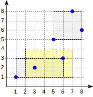
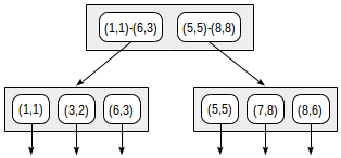
Now let's consider a very simple «one-level» example:
postgres=# create table points(p point);

postgres=# insert into points(p) values
  (point '(1,1)'), (point '(3,2)'), (point '(6,3)'),
  (point '(5,5)'), (point '(7,8)'), (point '(8,6)');

postgres=# create index on points using gist(p);
With this splitting, the index structure will look as follows:
The index created can be used to speed up the following query, for example: «find all points contained in the given rectangle». This condition can be formalized as follows:
p <@ box '(2,1),(6,3)' (operator <@ from «points_ops» family means «contained in»):postgres=# set enable_seqscan = off;
postgres=# explain(costs off) select * from points where p <@ box '(2,1),(7,4)';
                  QUERY PLAN
----------------------------------------------
 Index Only Scan using points_p_idx on points
   Index Cond: (p <@ '(7,4),(2,1)'::box)
(2 rows)
The consistency function of the operator ("indexed-field <@ expression", where indexed-field is a point and expression is a rectangle) is defined as follows. For an internal row, it returns «yes» if its rectangle intersects with the rectangle defined by the expression. For a leaf row, the function returns «yes» if its point («collapsed» rectangle) is contained in the rectangle defined by the expression.

The search starts with the root node. The rectangle (2,1)-(7,4) intersects with (1,1)-(6,3), but does not intersect with (5,5)-(8,8), therefore, there is no need to descend to the second subtree.
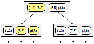
Upon reaching a leaf node, we go through the three points contained there and return two of them as the result: (3,2) и (6,3).
postgres=# select * from points where p <@ box '(2,1),(7,4)';
   p
-------
 (3,2)
 (6,3)
(2 rows)
Internals
Unfortunately, customary «pageinspect» does not allow looking into GiST index. But another way is available: «gevel» extension. It is not included in the standard delivery, so see the installation instructions.
If all is done right, three functions will be available to you. First, we can get some statistics:
postgres=# select * from gist_stat('airports_coordinates_idx');
                gist_stat
------------------------------------------
 Number of levels:          4            +
 Number of pages:           690          +
 Number of leaf pages:      625          +
 Number of tuples:          7873         +
 Number of invalid tuples:  0            +
 Number of leaf tuples:     7184         +
 Total size of tuples:      354692 bytes +
 Total size of leaf tuples: 323596 bytes +
 Total size of index:       5652480 bytes+

(1 row)
It is clear that the size of the index on airport coordinates is 690 pages and that the index consists of four levels: the root and two internal levels were shown in figures above, and the fourth level is leaf.
Actually, the index for eight thousand points will be considerably smaller: here it was created with a 10% fillfactor for clarity.
Second, we can output the index tree:
postgres=# select * from gist_tree('airports_coordinates_idx');
                                       gist_tree
-----------------------------------------------------------------------------------------
 0(l:0) blk: 0 numTuple: 5 free: 7928b(2.84%) rightlink:4294967295 (InvalidBlockNumber) +
     1(l:1) blk: 335 numTuple: 15 free: 7488b(8.24%) rightlink:220 (OK)                 +
         1(l:2) blk: 128 numTuple: 9 free: 7752b(5.00%) rightlink:49 (OK)               +
             1(l:3) blk: 57 numTuple: 12 free: 7620b(6.62%) rightlink:35 (OK)           +
             2(l:3) blk: 62 numTuple: 9 free: 7752b(5.00%) rightlink:57 (OK)            +
             3(l:3) blk: 72 numTuple: 7 free: 7840b(3.92%) rightlink:23 (OK)            +
             4(l:3) blk: 115 numTuple: 17 free: 7400b(9.31%) rightlink:33 (OK)          +
 ...
And third, we can output the data stored in index rows. Note the following nuance: the result of the function must be cast to the data type needed. In our situation, this type is «box» (a bounding rectangle). For example, notice five rows at the top level:
postgres=# select level, a from gist_print('airports_coordinates_idx')
  as t(level int, valid bool, a box) where level = 1;
 level |                                   a
-------+-----------------------------------------------------------------------
     1 | (47.663586,80.803207),(-39.2938003540039,-90)
     1 | (179.951004028,15.6700000762939),(15.2428998947144,-77.9634017944336)
     1 | (177.740997314453,73.5178070068359),(15.0664,10.57970047)
     1 | (-77.3191986083984,79.9946975708),(-179.876998901,-43.810001373291)
     1 | (-39.864200592041,82.5177993774),(-81.254096984863,-64.2382965088)
(5 rows)
Actually, the figures provided above were created just from this data.
Operators for search and ordering
Operators discussed so far (such as
<@ in the predicate p <@ box '(2,1),(7,4)') can be called search operators since they specify search conditions in a query.There is also another operator type: ordering operators. They are used for specifications of the sort order in ORDER BY clause instead of conventional specifications of column names. The following is an example of such a query:
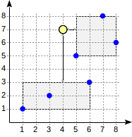
postgres=# select * from points order by p <-> point '(4,7)' limit 2;
   p
-------
 (5,5)
 (7,8)
(2 rows)
p <-> point '(4,7)' here is an expression that uses an ordering operator <->, which denotes the distance from one argument to the other one. The meaning of the query is to return two points closest to the point (4,7). Search like this is known as k-NN — k-nearest neighbor search.To support queries of this kind, an access method must define an additional distance function, and the ordering operator must be included in the appropriate operator class (for example, «points_ops» class for points). The query below shows operators, along with their types («s» — search and «o» — ordering):
postgres=# select amop.amopopr::regoperator, amop.amoppurpose, amop.amopstrategy
from pg_opclass opc, pg_opfamily opf, pg_am am, pg_amop amop
where opc.opcname = 'point_ops'
and opf.oid = opc.opcfamily
and am.oid = opf.opfmethod
and amop.amopfamily = opc.opcfamily
and am.amname = 'gist'
and amop.amoplefttype = opc.opcintype;
      amopopr      | amoppurpose | amopstrategy
-------------------+-------------+--------------
 <<(point,point)   | s           |            1  strictly left
 >>(point,point)   | s           |            5  strictly right
 ~=(point,point)   | s           |            6  coincides
 <^(point,point)   | s           |           10  strictly below
 >^(point,point)   | s           |           11  strictly above
 <->(point,point)  | o           |           15  distance
 <@(point,box)     | s           |           28  contained in rectangle
 <@(point,polygon) | s           |           48  contained in polygon
 <@(point,circle)  | s           |           68  contained in circle
(9 rows)
The numbers of strategies are also shown, with their meanings explained. It is clear that there are far more strategies than for «btree», only some of them being supported for points. Different strategies can be defined for other data types.
The distance function is called for an index element, and it must compute the distance (taking into account the operator semantics) from the value defined by the expression ("indexed-field ordering-operator expression") to the given element. For a leaf element, this is just the distance to the indexed value. For an internal element, the function must return the minimum of the distances to the child leaf elements. Since going through all child rows would be pretty costly, the function is permitted to optimistically underestimate the distance, but at the expense of reducing the search efficiency. However, the function is never permitted to overestimate the distance since this will disrupt the work of the index.
The distance function can return values of any sortable type (to order values, PostgreSQL will use comparison semantics from the appropriate operator family of «btree» access method, as described earlier).
For points in a plane, the distance is interpreted in a very usual sense: the value of
(x1,y1) <-> (x2,y2) equals the square root of the sum of squares of differences of the abscissas and ordinates. The distance from a point to a bounding rectangle is taken to be the minimal distance from the point to this rectangle or zero if the point lies within the rectangle. It is easy to compute this value without walking through child points, and the value is for sure no greater than the distance to any child point.Let's consider the search algorithm for the above query.

The search starts with the root node. The node contains two bounding rectangles. The distance to (1,1)-(6,3) is 4.0 and to (5,5)-(8,8) is 1.0.
Child nodes are walked through in the order of increasing the distance. This way, we first descend to the nearest child node and compute the distances to the points (we will show the numbers in the figure for visibility):

This information suffices to return the first two points, (5,5) and (7,8). Since we are aware that the distance to points that lie within the rectangle (1,1)-(6,3) is 4.0 or greater, we do not need to descend to the first child node.
But what if we needed to find the first three points?
postgres=# select * from points order by p <-> point '(4,7)' limit 3;
   p
-------
 (5,5)
 (7,8)
 (8,6)
(3 rows)
Although the second child node contains all these points, we cannot return (8,6) without looking into the first child node since this node can contain closer points (since 4.0 < 4.1).

For internal rows, this example clarifies requirements for the distance function. By selecting smaller distance (4.0 instead of actual 4.5) for the second row, we reduced the efficiency (the algorithm needlessly started examining an extra node), but did not break correctness of the algorithm.
Until recently, GiST was the only access method capable of dealing with ordering operators. But the situation has changed: RUM access method (to be discussed further) has already joined this group of methods, and it is not unlikely that good old B-tree will join them: a patch developed by Nikita Glukhov, our colleague, is being discussed by the community.
As of march 2019, k-NN support is added for SP-GiST in upcoming PostgreSQL 12 (also authored by Nikita). Patch for B-tree is still in progress.
R-tree for intervals
Another example of using GiST access method is indexing of intervals, for example, time intervals («tsrange» type). All the difference is that internal nodes will contain bounding intervals instead of bounding rectangles.
Let's consider a simple example. We will be renting out a cottage and storing reservation intervals in a table:
postgres=# create table reservations(during tsrange);

postgres=# insert into reservations(during) values
('[2016-12-30, 2017-01-09)'),
('[2017-02-23, 2017-02-27)'),
('[2017-04-29, 2017-05-02)');

postgres=# create index on reservations using gist(during);
The index can be used to speed up the following query, for example:
postgres=# select * from reservations where during && '[2017-01-01, 2017-04-01)';
                    during
-----------------------------------------------
 ["2016-12-30 00:00:00","2017-01-08 00:00:00")
 ["2017-02-23 00:00:00","2017-02-26 00:00:00")
(2 rows)
postgres=# explain (costs off) select * from reservations where during && '[2017-01-01, 2017-04-01)';
                                     QUERY PLAN
------------------------------------------------------------------------------------
 Index Only Scan using reservations_during_idx on reservations
   Index Cond: (during && '["2017-01-01 00:00:00","2017-04-01 00:00:00")'::tsrange)
(2 rows)
&& operator for intervals denotes intersection; therefore, the query must return all intervals intersecting with the given one. For such an operator, the consistency function determines whether the given interval intersects with a value in an internal or leaf row.Note that this is either not about getting intervals in a certain order, although comparison operators are defined for intervals. We can use «btree» index for intervals, but in this case, we will have to do without support of operations like these:
postgres=# select amop.amopopr::regoperator, amop.amoppurpose, amop.amopstrategy
from pg_opclass opc, pg_opfamily opf, pg_am am, pg_amop amop
where opc.opcname = 'range_ops'
and opf.oid = opc.opcfamily
and am.oid = opf.opfmethod
and amop.amopfamily = opc.opcfamily
and am.amname = 'gist'
and amop.amoplefttype = opc.opcintype;
         amopopr         | amoppurpose | amopstrategy
-------------------------+-------------+--------------
 @>(anyrange,anyelement) | s           |           16  contains element
 <<(anyrange,anyrange)   | s           |            1  strictly left
 &<(anyrange,anyrange)   | s           |            2  not beyond right boundary
 &&(anyrange,anyrange)   | s           |            3  intersects
 &>(anyrange,anyrange)   | s           |            4  not beyond left boundary
 >>(anyrange,anyrange)   | s           |            5  strictly right
 -|-(anyrange,anyrange)  | s           |            6  adjacent
 @>(anyrange,anyrange)   | s           |            7  contains interval
 <@(anyrange,anyrange)   | s           |            8  contained in interval
 =(anyrange,anyrange)    | s           |           18  equals
(10 rows)
(Except the equality, which is contained in the operator class for «btree» access method.)
Internals
We can look inside using the same «gevel» extension. We only need to remember to change the data type in the call to gist_print:
postgres=# select level, a from gist_print('reservations_during_idx')
as t(level int, valid bool, a tsrange);
 level |                       a
-------+-----------------------------------------------
     1 | ["2016-12-30 00:00:00","2017-01-09 00:00:00")
     1 | ["2017-02-23 00:00:00","2017-02-27 00:00:00")
     1 | ["2017-04-29 00:00:00","2017-05-02 00:00:00")
(3 rows)
Exclusion constraint
GiST index can be used to support exclusion constraints (EXCLUDE).
The exclusion constraint ensures given fields of any two table rows not to «correspond» to each other in terms of some operators. If «equals» operator is chosen, we exactly get the unique constraint: given fields of any two rows do not equal each other.
The exclusion constraint is supported by the index, as well as the unique constraint. We can choose any operator so that:
- It is supported by the index method — «can_exclude» property (for example, «btree», GiST, or SP-GiST, but not GIN).
- It is commutative, that is, the condition is met: a operator b = b operator a.
This is a list of suitable strategies and examples of operators (operators, as we remember, can have different names and be available not for all data types):
- For «btree»:
- «equals»
=
- «equals»
- For GiST and SP-GiST:
- «intersection»
&& - «coincidence»
~= - «adjacency»
-|-
- «intersection»
Note that we can use the equality operator in an exclusion constraint, but it is impractical: a unique constraint will be more efficient. That is exactly why we did not touch upon exclusion constraints when we discussed B-trees.
Let's provide an example of using an exclusion constraint. It is reasonable not to permit reservations for intersecting intervals.
postgres=# alter table reservations add exclude using gist(during with &&);
Once we created the exclusion constraint, we can add rows:
postgres=# insert into reservations(during) values ('[2017-06-10, 2017-06-13)');
But an attempt to insert an intersecting interval into the table will result in an error:
postgres=# insert into reservations(during) values ('[2017-05-15, 2017-06-15)');
ERROR: conflicting key value violates exclusion constraint "reservations_during_excl"
DETAIL: Key (during)=(["2017-05-15 00:00:00","2017-06-15 00:00:00")) conflicts with existing key (during)=(["2017-06-10 00:00:00","2017-06-13 00:00:00")).
«btree_gist» extension
Let's complicate the problem. We expand our humble business, and we are going to rent out several cottages:
postgres=# alter table reservations add house_no integer default 1;
We need to change the exclusion constraint so that house numbers are taken into account. GiST, however, does not support the equality operation for integer numbers:
postgres=# alter table reservations drop constraint reservations_during_excl;

postgres=# alter table reservations add exclude using gist(during with &&, house_no with =);
ERROR: data type integer has no default operator class for access method "gist"
HINT: You must specify an operator class for the index or define a default operator class for the data type.
In this case, "btree_gist" extension will help, which adds GiST support of operations inherent to B-trees. GiST, eventually, can support any operators, so why should not we teach it to support «greater», «less», and «equal» operators?
postgres=# create extension btree_gist;

postgres=# alter table reservations add exclude using gist(during with &&, house_no with =);
Now we still cannot reserve the first cottage for the same dates:
postgres=# insert into reservations(during, house_no) values ('[2017-05-15, 2017-06-15)', 1);
ERROR: conflicting key value violates exclusion constraint "reservations_during_house_no_excl"
However, we can reserve the second one:
postgres=# insert into reservations(during, house_no) values ('[2017-05-15, 2017-06-15)', 2);
But be aware that although GiST can somehow support «greater», «less», and «equal» operators, B-tree still does this better. So it is worth using this technique only if GiST index is essentially needed, like in our example.
RD-tree for full-text search
About full-text search
Let's start with a minimalist introduction to PostgreSQL full-text search (if you are in the know, you can skip this section).
The task of full-text search is to select from the document set those documents that match the search query. (If there are many matching documents, it is important to find the best matching, but we will say nothing about it at this point.)
For search purposes, a document is converted to a specialized type «tsvector», which contains lexemes and their positions in the document. Lexemes are words converted to the form suitable for search. For example, words are typically converted to lowercase, and variable endings are cut off:
postgres=# select to_tsvector('There was a crooked man, and he walked a crooked mile');
               to_tsvector
-----------------------------------------
 'crook':4,10 'man':5 'mile':11 'walk':8
(1 row)
We can also see that some words (called stop words) are totally dropped («there», «was», «a», «and», «he») since they presumably occur too often for search of them to make sense. All these conversions can certainly be configured, but that's another story.
A search query is represented with another type: «tsquery». Roughly, a query consists of one or several lexemes joint by connectives: «and» &, «or» |, «not»!.. We can also use parentheses to clarify operation precedence.
postgres=# select to_tsquery('man & (walking | running)');
         to_tsquery
----------------------------
 'man' & ( 'walk' | 'run' )
(1 row)
Only one match operator
@@ is used for full-text search.postgres=# select to_tsvector('There was a crooked man, and he walked a crooked mile') @@ to_tsquery('man & (walking | running)');
 ?column?
----------
 t
(1 row)
postgres=# select to_tsvector('There was a crooked man, and he walked a crooked mile') @@ to_tsquery('man & (going | running)');
 ?column?
----------
 f
(1 row)
This information suffices for now. We will dive a little deeper into full-text search in a next article that features GIN index.
RD-trees
For fast full-text search, firstly, the table needs to store a column of type «tsvector» (to avoid performing a costly conversion each time when searching) and secondly, an index must be built on this column. One of possible access methods for this is GiST.
postgres=# create table ts(doc text, doc_tsv tsvector);

postgres=# create index on ts using gist(doc_tsv);

postgres=# insert into ts(doc) values
  ('Can a sheet slitter slit sheets?'),
  ('How many sheets could a sheet slitter slit?'),
  ('I slit a sheet, a sheet I slit.'),
  ('Upon a slitted sheet I sit.'),
  ('Whoever slit the sheets is a good sheet slitter.'),
  ('I am a sheet slitter.'),
  ('I slit sheets.'),
  ('I am the sleekest sheet slitter that ever slit sheets.'),
  ('She slits the sheet she sits on.');

postgres=# update ts set doc_tsv = to_tsvector(doc);
It is, certainly, convenient to entrust a trigger with the last step (conversion of the document to «tsvector»).
postgres=# select * from ts;
-[ RECORD 1 ]----------------------------------------------------
doc     | Can a sheet slitter slit sheets?
doc_tsv | 'sheet':3,6 'slit':5 'slitter':4
-[ RECORD 2 ]----------------------------------------------------
doc     | How many sheets could a sheet slitter slit?
doc_tsv | 'could':4 'mani':2 'sheet':3,6 'slit':8 'slitter':7
-[ RECORD 3 ]----------------------------------------------------
doc     | I slit a sheet, a sheet I slit.
doc_tsv | 'sheet':4,6 'slit':2,8
-[ RECORD 4 ]----------------------------------------------------
doc     | Upon a slitted sheet I sit.
doc_tsv | 'sheet':4 'sit':6 'slit':3 'upon':1
-[ RECORD 5 ]----------------------------------------------------
doc     | Whoever slit the sheets is a good sheet slitter.
doc_tsv | 'good':7 'sheet':4,8 'slit':2 'slitter':9 'whoever':1
-[ RECORD 6 ]----------------------------------------------------
doc     | I am a sheet slitter.
doc_tsv | 'sheet':4 'slitter':5
-[ RECORD 7 ]----------------------------------------------------
doc     | I slit sheets.
doc_tsv | 'sheet':3 'slit':2
-[ RECORD 8 ]----------------------------------------------------
doc     | I am the sleekest sheet slitter that ever slit sheets.
doc_tsv | 'ever':8 'sheet':5,10 'sleekest':4 'slit':9 'slitter':6
-[ RECORD 9 ]----------------------------------------------------
doc     | She slits the sheet she sits on.
doc_tsv | 'sheet':4 'sit':6 'slit':2
How should the index be structured? Use of R-tree directly is not an option since it is unclear how to define a «bounding rectangle» for documents. But we can apply some modification of this approach for sets, a so-called RD-tree (RD stands for «Russian Doll»). A set is understood to be a set of lexemes in this case, but in general, a set can be any.
An idea of RD-trees is to replace a bounding rectangle with a bounding set, that is, a set that contains all elements of child sets.
An important question arises how to represent sets in index rows. The most straightforward way is just to enumerate all elements of the set. This might look as follows:

Then for example, for access by condition
doc_tsv @@ to_tsquery('sit') we could descend only to those nodes that contain «sit» lexeme: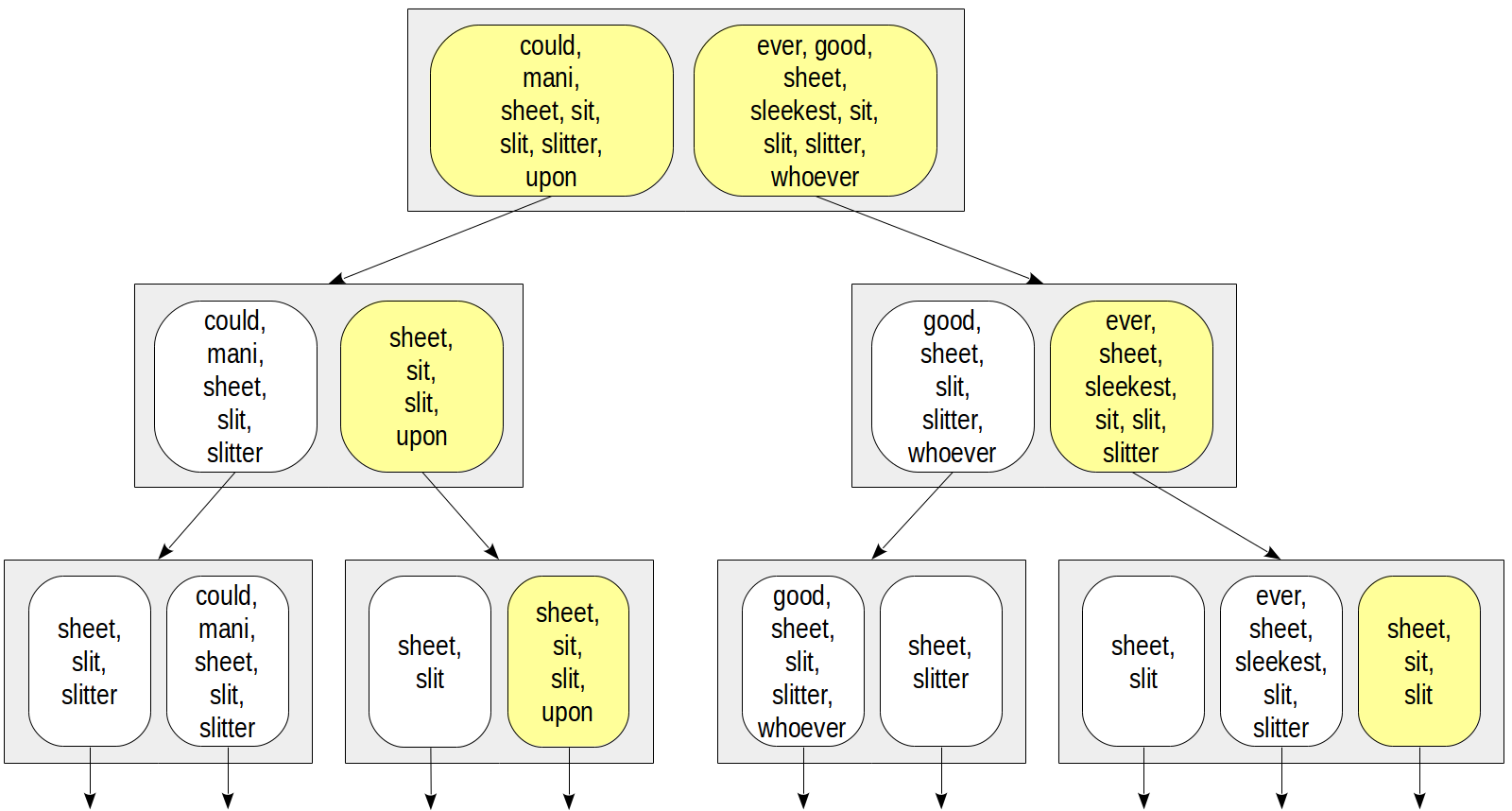
This representation has evident issues. The number of lexemes in a document can be pretty large, so index rows will have large size and get into TOAST, making the index far less efficient. Even if each document has few unique lexemes, the union of sets may still be very large: the higher to the root the larger index rows.
A representation like this is sometimes used, but for other data types. And full-text search uses another, more compact, solution — a so-called signature tree. Its idea is quite familiar to all who dealt with Bloom filter.
Each lexeme can be represented with its signature: a bit string of a certain length where all bits but one are zero. The position of this bit is determined by the value of hash function of the lexeme (we discussed internals of hash functions earlier).
The document signature is the bitwise OR of the signatures of all document lexemes.
Let's assume the following signatures of lexemes:
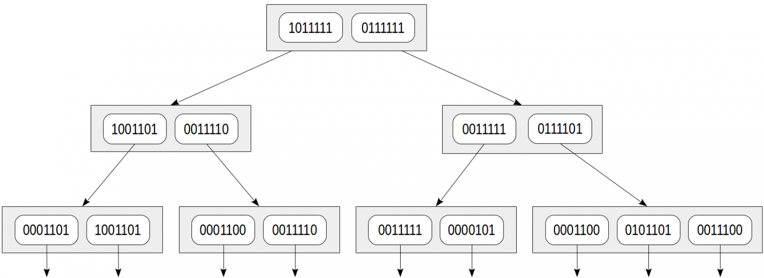
could    1000000
ever     0001000
good     0000010
mani     0000100
sheet    0000100
sleekest 0100000
sit      0010000
slit     0001000
slitter  0000001
upon     0000010
whoever  0010000
Then signatures of the documents are like these:
Can a sheet slitter slit sheets?                       0001101
How many sheets could a sheet slitter slit?            1001101
I slit a sheet, a sheet I slit.                        0001100
Upon a slitted sheet I sit.                            0011110
Whoever slit the sheets is a good sheet slitter.       0011111
I am a sheet slitter.                                  0000101
I slit sheets.                                         0001100
I am the sleekest sheet slitter that ever slit sheets. 0101101
She slits the sheet she sits on.                       0011100
The index tree can be represented as follows:
The advantages of this approach are evident: index rows have equal small sizes, and such an index is compact. But a drawback is also clear: the accuracy is sacrificed to compactness.
Let's consider the same condition
doc_tsv @@ to_tsquery('sit'). And let's compute the signature of the search query the same way as for the document: 0010000 in this case. The consistency function must return all child nodes whose signatures contain at least one bit from the query signature:
Compare with the figure above: we can see that the tree turned yellow, which means that false positives occur and excessive nodes are went through during the search. Here we picked up «whoever» lexeme, whose signature unfortunately was the same as the signature of «sit» lexeme. It's important that no false negatives can occur in the pattern, that is, we are sure not to miss needed values.
Besides, it may so happen that different documents will also get the same signatures: in our example, unlucky documents are «I slit a sheet, a sheet I slit» and «I slit sheets» (both have the signature of 0001100). And if a leaf index row does not store the value of «tsvector», the index itself will give false positives. Of course, in this case, the method will ask the indexing engine to recheck the result with the table, so the user will not see these false positives. But the search efficiency may get compromised.
Actually, a signature is 124-byte large in the current implementation instead of 7-bit in the figures, so the above issues are much less likely to occur than in the example. But in reality, much more documents get indexed as well. To somehow reduce the number of false positives of the index method, the implementation gets a little tricky: the indexed «tsvector» is stored in a leaf index row, but only if its size is not large (a little less than 1/16 of a page, which is about half a kilobyte for 8-KB pages).
Example
To see how indexing works on actual data, let's take the archive of «pgsql-hackers» email. The version used in the example contains 356125 messages with the send date, subject, author, and text:
fts=# select * from mail_messages order by sent limit 1;
-[ RECORD 1 ]------------------------------------------------------------------------
id         | 1572389
parent_id  | 1562808
sent       | 1997-06-24 11:31:09
subject    | Re: [HACKERS] Array bug is still there....
author     | "Thomas G. Lockhart" <Thomas.Lockhart@jpl.nasa.gov>
body_plain | Andrew Martin wrote:                                                    +
           | > Just run the regression tests on 6.1 and as I suspected the array bug +
           | > is still there. The regression test passes because the expected output+
           | > has been fixed to the *wrong* output.                                 +
           |                                                                         +
           | OK, I think I understand the current array behavior, which is apparently+
           | different than the behavior for v1.0x.                                  +
             ...
Adding and filling in the column of «tsvector» type and building the index. Here we will join three values in one vector (subject, author, and message text) to show that the document does not need to be one field, but can consist of totally different arbitrary parts.
fts=# alter table mail_messages add column tsv tsvector;

fts=# update mail_messages
set tsv = to_tsvector(subject||' '||author||' '||body_plain);
NOTICE:  word is too long to be indexed
DETAIL:  Words longer than 2047 characters are ignored.
...
UPDATE 356125
fts=# create index on mail_messages using gist(tsv);
As we can see, a certain number of words were dropped because of too large size. But the index is eventually created and can support search queries:
fts=# explain (analyze, costs off)
select * from mail_messages where tsv @@ to_tsquery('magic & value');
                        QUERY PLAN
----------------------------------------------------------
 Index Scan using mail_messages_tsv_idx on mail_messages
 (actual time=0.998..416.335 rows=898 loops=1)
   Index Cond: (tsv @@ to_tsquery('magic & value'::text))
   Rows Removed by Index Recheck: 7859
 Planning time: 0.203 ms
 Execution time: 416.492 ms
(5 rows)
We can see that together with 898 rows matching the condition, the access method returned 7859 more rows that were filtered out by rechecking with the table. This demonstrates a negative impact of the loss of accuracy on the efficiency.
Internals
To analyze the contents of the index, we will again use «gevel» extension:
fts=# select level, a
from gist_print('mail_messages_tsv_idx') as t(level int, valid bool, a gtsvector)
where a is not null;
 level |               a
-------+-------------------------------
     1 | 992 true bits, 0 false bits
     2 | 988 true bits, 4 false bits
     3 | 573 true bits, 419 false bits
     4 | 65 unique words
     4 | 107 unique words
     4 | 64 unique words
     4 | 42 unique words
...
Values of the specialized type «gtsvector» that are stored in index rows are actually the signature plus, maybe, the source «tsvector». If the vector is available, the output contains the number of lexemes (unique words), otherwise, the number of true and false bits in the signature.
It is clear that in the root node, the signature degenerated to «all ones», that is, one index level became absolutely useless (and one more became almost useless, with only four false bits).
Properties
Let's look at the properties of GiST access method (queries were provided earlier):
 amname |     name      | pg_indexam_has_property
--------+---------------+-------------------------
 gist   | can_order     | f
 gist   | can_unique    | f
 gist   | can_multi_col | t
 gist   | can_exclude   | t
Sorting of values and unique constraint are not supported. As we've seen, the index can be built on several columns and used in exclusion constraints.
The following index-layer properties are available:
     name      | pg_index_has_property
---------------+-----------------------
 clusterable   | t
 index_scan    | t
 bitmap_scan   | t
 backward_scan | f
And the most interesting properties are those of the column layer. Some of the properties are independent of operator classes:
        name        | pg_index_column_has_property
--------------------+------------------------------
 asc                | f
 desc               | f
 nulls_first        | f
 nulls_last         | f
 orderable          | f
 search_array       | f
 search_nulls       | t
(Sorting is not supported; the index cannot be used to search an array; NULLs are supported.)
But the two remaining properties, «distance_orderable» and «returnable», will depend on the operator class used. For example, for points we will get:
        name        | pg_index_column_has_property
--------------------+------------------------------
 distance_orderable | t
 returnable         | t
The first property tells that the distance operator is available for search of nearest neighbors. And the second one tells that the index can be used for index-only scan. Although leaf index rows store rectangles rather than points, the access method can return what's needed.
The following are the properties for intervals:
        name        | pg_index_column_has_property
--------------------+------------------------------
 distance_orderable | f
 returnable         | t
For intervals, the distance function is not defined and therefore, search of nearest neighbors is not possible.
And for full-text search, we get:
        name        | pg_index_column_has_property
--------------------+------------------------------
 distance_orderable | f
 returnable         | f
Support of index-only scan has been lost since leaf rows can contain only the signature without the data itself. However, this is a minor loss since nobody is interested in the value of type «tsvector» anyway: this value is used to select rows, while it is source text that needs to be shown, but is missing from the index anyway.
Other data types
Finally, we will mention a few more types that are currently supported by GiST access method in addition to already discussed geometric types (by example of points), intervals, and full-text search types.
Of standard types, this is the type "inet" for IP-addresses. All the rest is added through extensions:
- cube provides «cube» data type for multi-dimensional cubes. For this type, just as for geometric types in a plane, GiST operator class is defined: R-tree, supporting search for nearest neighbors.
- seg provides «seg» data type for intervals with boundaries specified to a certain accuracy and adds support of GiST index for this data type (R-tree).
- intarray extends the functionality of integer arrays and adds GiST support for them. Two operator classes are implemented: «gist__int_ops» (RD-tree with a full representation of keys in index rows) and «gist__bigint_ops» (signature RD-tree). The first class can be used for small arrays, and the second one — for larger sizes.
- ltree adds «ltree» data type for tree-like structures and GiST support for this data type (RD-tree).
- pg_trgm adds a specialized operator class «gist_trgm_ops» for use of trigrams in full-text search. But this is to be discussed further, along with GIN index.
Read on.
